Anand Asthagiri
Department of Bioengineering
Northeastern University
Boston, MA
Copyright ©2018 Anand Asthagiri. All rights reserved
- 1 Preface
- 2 Quantifying and modeling reaction progress
- 3 First-order reactions
- 3.1 Half-life
- 4 Second-order reactions
- 5 Unpacking the rate constant
- 6 Chemical equilibrium vs steady state
- 6.1 Steady state
- 6.2 Chemical equilibrium
- 7 Insights into the origins of chemical equilibrium criteria
- 8 Simultaneous reactions in biological systems
- 9 Sequential reactions and yield
- 10 Competing reactions
- 11 Reversible binding reaction
- 12 Graphical analysis of a non-linear first-order system
- 13 Simple receptor-ligand binding
- 13.1 Dimensional analysis
- 14 Predicting the dynamics of simple receptor-ligand binding
- 15 The rate-limiting step: simplifying models of reaction systems
- 16 Enzymes: an introduction
1 Preface
My students have used this textbook as an online resource in my Biomolecular Dynamics and Control class since the founding of the Bioengineering department at Northeastern University in 2013. I give my deepest thanks to the many students who have given me input and feedback during the formative stages of the book. The book evolved rapidly during the first 5 years and reached its present form in 2018. I view it as a living textbook, and should you have suggestions or corrections, I welcome your input.
Anand Asthagiri
2 Quantifying and modeling reaction progress
2.1 Why we need to quantify reaction progress
How far has a reaction gone? The reaction might be one that yields a pharmaceutical that we seek to produce efficiently. The reaction could be generation of an unwanted waste product or toxin.
As an example, consider a biomolecular reaction where a receptor R on a cell surface binds and detects a ligand L in the environment. Together, they form a complex C. We write the reaction as:
\begin{equation} \ce{R + L -> C} \label{rxn:toxin-R} \end{equation}
Receptor-ligand binding is a prominent mechanism for cell-to-cell communication. It is how hormones, a type of ligand, secreted in a gland trigger responses in distant target cells in other organs: the cells have receptors for the hormones. Ligands can also be produced locally in a tissue and the source does not have to be our own cells. Bacterial infections result in the release of bacterial components, such as lipopolysaccharide (LPS). Receptors on our cells bind LPS and trigger a wide range of responses.
Suppose L is a toxin and the formation of C by reaction \ref{rxn:toxin-R} drives cell death. We may seek to prevent L from binding its receptor. One strategy is to flood the tissue with a decoy D that will bind and ``soak up'' L through the reaction:
\begin{equation} \ce{L + D -> LD} \label{rxn:toxin-D} \end{equation}
where LD is a heterodimer. With L sequestered in LD heterodimers, L cannot bind and activate the receptor R.
As an engineer designing this therapeutic strategy, we need to size up a host of questions, including:
- how quickly does the toxin L bind the receptor R?
- how much decoy D will be needed to compete against L binding to R?
- how far along is the adverse reaction \eqref{rxn:toxin-R} in a patient?
- for a particular level of infection (e.g., concentration of C in the body), how much more of the favorable reaction \ref{rxn:toxin-D} is occurring compared to the adverse reaction?
To begin to evaluate these and related questions, we need a way to quantify how far a reaction has progressed. We need a metric, for example, to assess how far a desirable reaction (e.g., \eqref{rxn:toxin-D}) has gotten compared to its undesirable counterpart (\ref{rxn:toxin-R}).
With a way to monitor and keep track of reaction progress, we could develop a model of how far each reaction progresses over time (dynamics/kinetics) or what might happen if we wait a really long time for things to ``settle down'' (equilibrium)1. We could then model different scenarios and predict a proper dose of decoy for different levels of toxin exposure.
2.2 How we quantify reaction progress: extent of reaction
Extent of reaction for a simple reaction
Consider a single simple bimolecular2 reaction \(\ce{A + B -> AB}\), we define a metric, the extent of reaction \((\xi)\), based on the quantity of a reaction species present now, relative to when the reaction started. That is,
\begin{align} \xi & = \{\mathrm{moles\ of\ AB\ now}\} - \{\mathrm{initial\ moles\ of\ AB}\} \\ %\notag & = n_{AB} - n_{AB}^o \label{eq:xiAB} \end{align}
where \(n_i\) refers to the amount of species \(i\) in units of moles (mol) or numbers of molecules (#). Recall that Avogadro’s number (\(6.022\times10^{23}\) #/mol) is used to convert between moles and numbers of molecules.
It is seems reasonable to expect that for one reaction, there ought to be just one value for the extent of reaction. That is, it shouldn’t depend on whether \(\xi\) is calculated using amounts of species AB, A or B. Regardless of which species we use to quantify reaction progress, we should get the same answer. File this away: one \(\xi\) per reaction.
If we were to use the amount of A to calculate \(\xi\), our formula would be similar, in spirit, but with an important difference:
\begin{align} \xi & = - \{\mathrm{moles\ of\ A\ now}\} - \{\mathrm{initial\ moles\ of\ A}\} \\ & = - (n_{A} - n_{A}^o) \label{eq:xiA} \end{align}
Can you spot the difference between Eqs. \ref{eq:xiA} vs. \ref{eq:xiAB}? The negative sign in Eq. \ref{eq:xiA} is critical. As the reaction proceeds, for every molecule of AB produced, one molecule of A is consumed. Therefore, the amount of A present now will be less than the initial amount of A. The difference \(\{\mathrm{moles\ of\ A\ now}\} - \{\mathrm{initial\ moles\ of\ A}\})\) will be negative, whereas the same difference calculated with the amounts of AB will be positive. The negative sign in Eq. \ref{eq:xiA} is necessary when reagents are used to calculate the extent of reaction.
Another wrinkle in calculating extent of reaction: stoichiometric factors
We have seen that the formula for calculating extent of reaction changes by a sign factor when using the the amount of reagent versus product.
The situation can in fact get slightly more complicated. Consider a reaction where two molecules of \(\mathrm{A}\) come together to form a dimer \(\mathrm{A_2}\). This is a homodimerization: \[ \ce{2 A -> A_2} \label{rxn:homodimer}\] Now, for every molecular of \(A_2\) produced, two molecules of \(A\) are consumed. The stoichiometric ratio of \(A\) to \(A_2\) is 2:1.
We still have only one reaction. Therefore, there can be only one extent of reaction. Our metric of how far the reaction has progressed cannot depend on which species in the reaction we are talking about.
The way we calculate extent of reaction must therefore take into account whether the species not only is a reagent or product, but also its stoichometry in the reaction. You might guess how; the answer is next.
Extent of reaction: the general case
Consider a balanced reaction
\[\ce{aA + bB -> cC + dD}\]
where a, b, c and d are absolute values of stoichiometric factors that balance atomic species on the reagent and product sides.
The extent of reaction is:
\begin{equation} \xi = \frac{n_A - n_A^o}{\nu_a} = \frac{n_B - n_B^o}{\nu_b} = \frac{n_C - n_C^o}{\nu_c} = \frac{n_D - n_D^o}{\nu_d} \label{eq:xi_general} \end{equation}
where the denominators are the stoichometric factors of each species, written as \(\nu_a = -a\), \(\nu_b = -b\), \(\nu_c = c\), and \(\nu_d = d\).
Note that the stoichiometric factor is negative for a reagent and positive for a product.
In more compact form, we can write
\begin{equation} \xi = \frac{n_i - n_i^o}{\nu_i} \label{eq:xi_compact} \end{equation}
with \(\nu_i < 0\) for reagent i or \(\nu_i > 0\) for product i.
2.3 Rate of reaction
Having now a way to quantify extent of reaction (\(\xi\)), we can now think about how fast a reaction is progressing. How does \(\xi\) change in time? Does the reaction accelerate, i.e., \(\xi\) increase with time? Perhaps, the reaction is slowing down over time, i.e., \(\xi\) decreases with time.
For any property \(X\), how \(X\) changes with time is given by its time-derivative. Applying this idea, the rate of reaction — sometimes called the velocity of reaction — is \({d\xi}/{dt}\).
We can go a bit further and replace \(\xi\) with the amount of species i:
\begin{equation} \frac{d\xi}{dt} = \frac{d}{dt}\left(\frac{n_i-n_i^o}{\nu_i}\right) \end{equation}
Because the initial amount of species \(i\) and its stoichiometric factor are constants, this simplifies to:
\begin{equation} \frac{d\xi}{dt} = \frac{1}{\nu_i} \frac{dn_i}{dt} \label{eq:raterxn} \end{equation}
The rate of reaction is the rate at which moles of species change with time, adjusted for the stoichiometric coefficient. With this adjustment, it does not matter which reaction species is used to quantify reaction rate: each reaction has a single rate.
Equation (\ref{eq:raterxn}) provides a way to quantify the rate of reaction. If we measure the amount of species \(i\) over time, we could calculate the derivative and determine the rate of reaction. This is the empirical way.
Could we, without doing experiments and taking measurements, model and predict the rate of a reaction? That is, given a reaction, such as \(\ce{2 A -> A_2}\), is there a way to express mathematically (model) how the rate of reaction might depend on properties of the molecular system? For example, it is reasonable to expect that the rate of reaction might depend on the amounts of reacting species (\(n_i\)) in some way. Little reagent, slow reaction; lots of reagent, very fast reaction. For a special class of reactions, we can propose a physically-reasonable way to model the rate of reaction, and we go there next.
2.4 Elementary reactions
For a certain class of reactions known as elementary reactions, we can model the rate of reaction based on physical insights at the molecular level. Elementary reactions are unique in that they represent a single molecular event. For example, the docking or binding of an enzyme (E) to its substrate (S)
\begin{equation} \ce{E + S -> ES} \label{rxn:E-Sdock} \end{equation}
can be viewed as an elementary reaction with a molecularity of two.
Because elementary reactions represent single molecular events, it is difficult to contemplate — from a physical perspective — an elementary reaction that has more than two reagents3. Thus, the molecularity — a term used only for elementary reactions — is very rarely greater than 2 and never greater than 3.
Reaction (\ref{rxn:E-Sdock}) is just the first step in a sequence of molecular events that leads to a product (P). If one includes the subsequent steps4 and writes a composite reaction of substrate conversion to product, then we would have the following non-elementary reaction:
\begin{equation} \ce{E + S -> E + P} \label{rxn:E-S-P} \end{equation}
Note that reaction \ref{rxn:E-S-P} has only two reagents (E and S), as did reaction \ref{rxn:E-Sdock}. Just because a reaction has 2 or fewer reagents does not make it an elementary reaction. The reaction must be a single molecular event in order to be elementary.
An elementary reaction is not a composite of many molecular steps. For example, cellular respiration of glucose is described by the reaction \(\ce{C6H12O6 + 6 O2 -> 6 H2O + 6 CO2}\). This is not an elementary reaction since the reaction of glucose with oxygen is not a single molecular event, but one that occurs through a series of molecular interactions/steps. Indeed, if one were to consider this a single molecular event, it would require one molecule of glucose to encounter and interact with six molecules of oxygen at a single point in space and time. The likelihood of a seven-member intermolecular encounter is zero.
2.5 Law of mass action
A basic requirement for an elementary reaction to occur is that the reagents, say A and B, must come close enough to react. A and B are moving around randomly in a reaction volume (\(V_R\)). How often they come close enough, i.e., ``collide'' at a molecular lengthscale, depends on a number of factors. Among them, two basic considerations are how many A and B molecules are present and how much space (or volume) is available for the molecules.
The frequency of collisions will be greater if there are more molecules of A and B. With more A and B per unit volume, they are more likely to bump into one another as they move around randomly. Thus, ``packing'' more reagents in a volume should drive up the frequency of collisions and thereby increase the rate of reaction in that volume. This physical model leads us to the Law of Mass Action, expressed mathematically as
\begin{equation} \frac{1}{V_R} \frac{d\xi}{dt} \propto \mathrm{[A][B]} \label{eq:mass-action-proportional} \end{equation}
The Law of Mass Action (\ref{eq:mass-action-proportional}) states that the rate of reaction per unit volume is proportional to the product of reagent concentrations for an elementary reaction. Note proportional but not equal. Proportionality suggests that frequency of collisions alone does not tell the whole story of reaction.
Even if an A molecule physically comes close enough to interact with B, what’s the chance that encounter will actually result in a product? After all, what if they come together in the wrong orientation? One can imagine that it is probably nonproductive if the reactive region of A isn’t facing B when they happen to encounter each other. And, do they bring sufficient energy to make the reaction possible? These considerations of configuration and energetics mean that only a fraction of collisions will successfully react. The probability that any individual collision will actually yield a reaction product contributes to the proportionality constant suggested in Eq. \ref{eq:mass-action-proportional}. The proportionality constant is referred to as the rate constant, \(k\), and using it, we can write the Law of Mass Action as:
\begin{equation} \frac{1}{V_R} \frac{d\xi}{dt} = k \mathrm{[A][B]} \label{eq:mass-action} \end{equation}
For an elementary reaction with reagent A and a molecularity of 1, the rate of reaction depends on the concentration of only one reagent:
\begin{equation} \frac{1}{V_R} \frac{d\xi}{dt} = k \mathrm{[A]} \label{eq:mass-action-molec1} \end{equation}
2.6 Putting together the pieces
We have now the definition of extent of reaction (Eq. \ref{eq:xi_compact}). We also have a physical model — the Law of Mass Action (Eq. \ref{eq:mass-action}) for how the extent of reaction changes in time based on current reaction conditions, namely the volume and amounts of reagents.
Inserting our expression for \(\xi\) from \ref{eq:xi_compact} into the Law of Mass Action gives us:
\begin{align} \frac{1}{V_R} \frac{d\xi}{dt} & = k \mathrm{[A][B]} \\ \frac{1}{V_R} \frac{d\left(\frac{n_i - n_i^o}{\nu_i}\right)}{dt} & = k \mathrm{[A][B]} \\ \end{align}
where \(i\) refers to any of the species in the elementary bimolecular reaction \(\ce{A + B -> \mathrm{products}}\). Since \(n_i^o\) and \(\nu_i\) do not change in time, we can simplify the above to
\begin{align} \frac{1}{\nu_i} \frac{dn_i}{dt} & = k \mathrm{[A][B]} V_R\\ \label{eq:ratelaw} \end{align}
This equations tells us that if we know the present condition (concentrations of A and B and the volume \(V_R\)) and we know the reaction (and therefore \(\nu_i\)), we can predict the amount of any species in the reaction \(n_i\) over time. This is at the heart of what we do in the next chapter, as we apply the Law of Mass Action to different reaction systems.
3 First-order reactions
Elementary reactions with a single reagent are ubiquitous in biology. Unbinding or dissociation is a prime example. Instances include the unbinding of a ligand from its receptor or the release of a product from an enzyme-substrate complex. The reaction, in general, is represented as follows:
\begin{equation} \ce{C -> A + B} \label{rx:unimolecular} \end{equation}
Having a single reagent, the reaction is referred to as having a molecularity of one. The term molecularity is reserved for elementary reactions, as these reactions represent a discrete molecular event.
For the unimolecular elementary reaction in \ref{rx:unimolecular}, the Law of Mass Action models the rate of reaction as:
\begin{equation} \frac{1}{V_R} \frac{d\xi}{dt} = k [C] \label{eq:firstOrderRate} \end{equation}
In contrast to elementary reactions, composite reactions are the sum of two or more molecular steps. For example, the aerobic respiration of glucose to produce water and carbon dioxide occurs through many reaction steps. We typically see these steps depicted in a complex chart of molecules and arrows involving glycolysis, Krebs' cycle and oxidative phosphorylation. Even the individual reactions shown in the diagram are themselves composed of elementary molecular steps. The point here is that these are examples of composite reactions for which the term molecularity is not applied.
In some cases, composite reactions may also follow a simple rate law that resembles \ref{eq:firstOrderRate}. That is, the rate of reaction progress is related to the concentration of a single reagent raised to the first power. Reactions whose rate is linearly proportional to a single reagent concentration are referred to as first-order reactions.
While Eq. \ref{eq:firstOrderRate} tells us the rate at which reaction progresses (\(d\xi/dt\)), we usually are interested in predicting how the amounts of reaction species changes over time (\(dn_i/dt\)). Recall that \(\xi\) can be expressed in terms of any of the species in the reaction. For example, \(\xi = \left(n_C - n_C^o\right)/\nu_C\) where the stoichiometric factor for C is -1. Substituting this expression for \(\xi\) into Eq. \ref{eq:firstOrderRate}, we write:
\begin{equation} \frac{1}{V_R} \frac{dn_C}{dt} = - k [C] \label{eq:rateVarV} \end{equation}
Since \(n_C^o\) is a constant, it is eliminated from the time-derivative. The negative on the right hand side of Eq. \ref{eq:rateVarV} comes from inserting \(-1\) for \(\nu_C\).
Comparing Eqs. \ref{eq:firstOrderRate} and \ref{eq:rateVarV} shows that we have converted a statement about the rate of reaction progress into a model for the rate of change in moles of C. The latter is more directly useful, as we are typically interested in knowing how amounts of species change over time due to reaction(s).
Can we solve Eq. \ref{eq:rateVarV}? Not quite. Eq. \ref{eq:rateVarV} contains more than one time-dependent variable. Volume \(V_R\) could change over the course of a reaction, particularly for a reaction occurring in the gas phase. For a simple ideal-gas, the Ideal Gas Law \(pV=nRT\) states that volume \(V\) is proportional to moles of species (\(n\)) at fixed pressure \(p\) and temperature \(T\). Thus, if the stoichiometry of the reaction indicates that more products will be formed than reagents, the reaction volume will expand; the converse is true if fewer species are products than reagents. Reaction \ref{rx:unimolecular} presently under consideration produces one more product species than reagents. If it were occuring in the gas phase, we would expect volume to increase during the course of the reaction. Liquids are incompressible under standard pressure conditions in which biological systems are studied, and one can reasonably assume that volume for liquid-phase reactions is constant during the course of reaction.
Suppose this is a liquid-phase reaction and volume is constant. We can bring \(V_R\) inside the time-derivative and rewrite as
\begin{equation} \frac{d(n_C/V_R)}{dt} = \frac{d[C]}{dt} = -k [C] \label{eq:rateConstV} \end{equation}
where the amount (\(n_C\)) is converted to concentration (\([C]\)) within the time-derivative. This simplification leaes us with a differential equation with a single time-dependent variable \([C]\). With the initial condition that \(C = C_o\) at \(t=0\), the solution is5:
\begin{equation} C = C_o e^{-kt} \label{eq:firstOrderSoln} \end{equation}
The concentration of C is predicted to decrease exponentially over time from its initial concentration \([C]_o\) and approaches \(0\) in the long run. ``How long do we have to wait?'' one might ask. That depends on the value of the rate constant \(k\). The larger the rate constant, the quicker C is depleted and the shorter the lifetime of C. If this qualitative reply is unsatisfactory, a more quantitative answer lies in calculating how long it takes for half the reagent to be consumed.
3.1 Half-life
The half-life (\(t_{1/2}\)) is the time it takes for the reagent to depelete to half of its initial concentration. For a first-order reaction, we use the solution \ref{eq:firstOrderSoln} to solve for the time \(t\) at which \(C = C_o/2\) and obtain:
\begin{equation} t_{1/2} = \frac{\ln{2}}{k} \label{eq:halfLifeFirst} \end{equation}
Thus, the half-life of a first-order process does not depend on the starting concentration of the reagent. The half-life depends only on \(k\).
4 Second-order reactions
If first-order elementary reactions involving dissociation or unbinding are prevalent in biology, it stands to reason that the opposite process — association or binding of two molecules — is also widespread. Indeed, ligand binding to receptor to form a complex is a pervasive means for biological communication. Enzyme binding to substrate to form an enzyme-substrate complex is the first step in enzyme catalysis of substrate conversion to product.
These reactions generally have the form:
\begin{equation} \ce{A + B -> \mathrm{products}} \label{rx:2ndOrder} \end{equation}
If the reaction is elementary, we can model the dynamics of the reaction by applying the Law of Mass Action. The rate of reaction is:
\begin{equation} \frac{d\xi}{dt} = k A B V_R \label{eq:ratelaw2ndorder} \end{equation}
The issue is that we have one equation with three time-dependent variables (\(\xi\), \(A\) and \(B\)). If we focus on deriving \(A\) first, we need some way to put \(\xi\) and \(B\) in terms of \(A\).
To begin, let’s focus on replacing \(d\xi/dt\) with \(dA/dt\). Recall that \(\xi\) is related to the moles of A:
\begin{equation} \xi = \frac{n_A-n_A^o}{\nu_A} % leave out for now: = \frac{n_B-n_B^o}{\nu_B} \label{eq:xi_relate_AandB} \end{equation}
where \(n_A^o\) is the moles of A at initial time.
Since \(A = n_\mathrm{A}/V_R\) and assuming a constant-volume reaction (\(V_R = V_{Ro}\)), \eqref{eq:xi_relate_AandB} simplifies to:
\begin{equation} \xi = \frac{AV_R - A_oV_R^o}{\nu_A} = \frac{V_R}{\nu_A} \left( A - A_o \right) \label{eq:xi_concA} \end{equation}
Using the above equation, we can replace \(\xi\) with \(A\) in \ref{eq:ratelaw2ndorder} to obtain:
\begin{align} \frac{V_R}{\nu_A} \frac{d(A-A_o)}{dt} & = k AB V_R \\ \frac{d(A-A_o)}{dt} & = \nu_A k AB \end{align}
Observe that \(dA_o/dt = 0\). Thus,
\begin{align} \frac{dA}{dt} & = \nu_A k AB \label{eq:rateA} \end{align}
Equation \ref{eq:rateA} gives us the rate of change in concentration of A. It is worthwhile to take a moment to compare this equation to the rate of reaction \ref{eq:ratelaw2ndorder}. Note that the stoichiometry of the species appears in the equation for the rate of change in concentration of A. This should make intuitive sense. Whereas \ref{eq:ratelaw2ndorder} describes a reaction-property (\(\xi\)), \eqref{eq:rateA} represents a property for an individual species A.
Of course, \(\nu_A = -1\) and we write:
\begin{equation} \frac{dA}{dt} = - k A B \label{eqch2_2:step5} \end{equation}
We’ve made some progress. We are now faced with two (instead of three) time-dependent variables, \(A\) and \(B\), with still only one equation. To proceed, we need to put \(B\) in terms of \(A\). We can use the fact that changes in the moles or concentration of A are related to the changes in moles or concentration of B, as follows:
\begin{align} \xi = \frac{n_A-n_A^o}{\nu_A} &= \frac{n_B-n_B^o}{\nu_B} \label{eq:xi_concAB} \\ \frac{A-A_o}{\nu_A} &= \frac{B - B_o}{\nu_B} \label{eq:concA_concB} \end{align}
Note that in going from \eqref{eq:xi_concAB} to \eqref{eq:concA_concB}, we applied again the assumption that volume is constant. The reasoning is the same as above, when we simplified \eqref{eq:xi_relate_AandB} to \eqref{eq:xi_concA}.
Rearranging \eqref{eq:concA_concB}, \(B = B_o + \left(A - A_o\right)\). Substituting in \eqref{eqch2_2:step5}, we get
\begin{equation} -\frac{dA}{dt} = k A \left( B_o + \left(A - A_o\right) \right) \label{eq:ArelateB} \end{equation}
We have now one equation with one time-dependent variable \(A\). Now, it is simply a matter of integrating to derive \(A(t)\). The stepwise solution is provided below:
\begin{align} \frac{dA}{A \left( B_o + \left(A - A_o\right) \right)} &= -k dt \\ \int_{A_o}^{A}\frac{dA}{A \left( B_o + \left(A - A_o\right) \right)} &= -k \int_{o}^{t}dt \label{eqch2_2:step7} \end{align}
Apply partial fraction expansion to solve the integral on the left. When \(A_o \ne B_o\), we want to find \(\alpha\) and \(\beta\) that satisfy:
\begin{equation} \frac{1}{A \left( B_o + \left(A - A_o\right) \right)} = \frac{\alpha}{A} + \frac{\beta}{B_o + \left(A - A_o\right)} \label{eqch2_2:step8} \end{equation}
After adding the fractions on the right side, we find that its numerator must equal 1:
\begin{equation} \alpha \left( B_o + \left(A - A_o\right) \right) + \beta A = 1 \end{equation}
which means the following system of equations must be satisfied:
\begin{align} \alpha + \beta &= 0 \\ \alpha \left( B_o - A_o \right) &= 1 \end{align}
Therefore, \(\alpha = 1/ \left( B_o - A_o \right)\) and \(\beta = -1/ \left(B_o - A_o\right)\) where \(A_o \ne B_o\).
Using these results in \eqref{eqch2_2:step8}, equation \eqref{eqch2_2:step7} can be rewritten as:
\begin{gather*} \int_{A_o}^{A} \frac{\alpha}{A} + \frac{\beta}{B_o + \left(A - A_o\right)} dA = -k \int_{o}^{t}dt\\ \\ \int_{A_o}^{A} \left( \frac{1/ \left( B_o - A_o \right)}{A} + \frac{-1/ \left(B_o - A_o\right)}{B_o + \left(A - A_o\right)} \right) dA = -k \int_{o}^{t}dt\\ \\ \int_{A_o}^{A} \frac{1/ \left( B_o - A_o \right)}{A} dA - \int_{A_o}^{A} \frac{1/ \left(B_o - A_o\right)}{B_o + \left(A - A_o\right)} dA = -k \int_{o}^{t}dt \\ \\ \frac{1}{B_o - A_o} \int_{A_o}^{A} \frac{1}{A} dA - \frac{1}{B_o - A_o} \int_{A_o}^{A} \frac{1}{B_o + \left(A - A_o\right)} dA = -k \int_{0}^{t}dt \\ \\ \frac{1}{B_o - A_o} \Big( \ln{\left( A \right)} - \ln{\big( B_o + \left(A - A_o\right) \big)} \Big) \Big|_{A_o}^A = -kt \\ \\ \frac{1}{B_o - A_o} \ln{\left( \frac{A}{B_o + \left(A - A_o\right)}\right)} \Big|_{A_o}^A = -kt\\ \\ \frac{1}{B_o - A_o} \ln{\left( \frac{A}{B_o + \left(A - A_o\right)}\right)} - \ln{\left( \frac{A_o}{B_o}\right)} = -kt \end{gather*}
Finally, we have:
\begin{equation} \frac{1}{A_o - B_o} \ln{\left( \frac{B_o}{A_o} \frac{A}{B_o + \left(A - A_o\right)}\right)} = kt \label{eq:almostDone} \end{equation}
Recalling from Eq. \ref{eq:ArelateB} that \(B_o + \left(A - A_o\right)\) is in fact \(B\), a simple implicit form of the solution is:
\begin{equation} \frac{1}{A_o - B_o} \ln{\left( \frac{B_o}{A_o} \frac{A}{B}\right)} = kt \label{eq:implicitSoln} \end{equation}
An explicit form of solution for \(A(t)\) can also be derived from \ref{eq:almostDone} as follows:
\begin{gather*} \ln{\left( \frac{B_o}{A_o} \frac{A}{B_o + \left(A - A_o\right)}\right)} = \left(A_o - B_o\right) kt \\ \\ \frac{B_o}{A_o} \frac{A}{B_o + \left(A - A_o\right)} = e^{ \left(A_o - B_o\right) kt } \\ \\ \frac{A_o}{B_o} \frac{B_o + \left(A - A_o\right)}{A} = e^{ - \left(A_o - B_o\right) kt } \\ \\ \frac{B_o + \left(A - A_o\right)}{A} = \frac{B_o}{A_o} e^{ - \left(A_o - B_o\right) kt } \\ \\ B_o - A_o = A \frac{B_o}{A_o} e^{ - \left(A_o - B_o\right) kt } - A \\ \\ A = \frac{B_o - A_o}{ \frac{B_o}{A_o} e^{- \left(A_o - B_o\right) kt} - 1} \\ \\ A = A_o \frac{B_o - A_o}{B_o e^{- \left(A_o - B_o\right) kt } - A_o} \end{gather*}
This solution holds for the general case when \(A_o \ne B_o\). If A and B are provided initially in stoichiometric amounts, then we must return to \ref{eq:ArelateB} and solve under the condition that \(A_o = B_o\), as detailed in the following example.
4.1 Example: Equimolar second-order elementary reaction and half-life
Consider a constant-volume elementary reaction in which A and B are provided initially at equimolar concentration. Predict the time-evolution of reagent concentrations. Does it take longer to reach half the initial concentration of reagents if the reaction is started with more reagents?
Solution
The reaction given is \(\ce{A + B -> \mathrm{products}}\). We are also told that the reaction starts with equimolar concentration of A and B. Hence, \(A_o = B_o\). For this reaction, equimolar concentration also means stoichiometric amounts of reagents. That it, the ratio of initial amounts of A and B match the 1:1 stoichiometry of the species in the reaction. With reagents supplied at stoichiometric amounts, they will run out together when the reaction completes, i.e., there is no limiting reagent.
Our initial approach might be to use equation \ref{eq:implicitSoln} that we just derived. However, this equation fails when using \(A_o = B_o\). To develop the solution, we need to apply \(A_o = B_o\) to the differential equation \ref{eq:ArelateB} for the rate of change in \(A\). The governing rate equation becomes:
\begin{equation} \frac{dA}{dt} = -k A^2 \end{equation}
The solution is derived by separation of variables and integration:
\begin{gather*} \int_{A_o}^{A} \frac{dA}{A^2} = -k \int_0^t dt \\ \\ \left(\frac{1}{A} - \frac{1}{A_o}\right) = k t \end{gather*}
The final solution is:
\begin{equation} A = \frac{A_o}{1+kA_ot} \label{eq:equimolar} \end{equation}
Since A and B were provided initially in equimolar amount, the concentration of B follows the same time-course as that of A.
The second part of the question asks whether it will take longer to deplete half the reagent if we start with more. The time to deplete half the reagent is determined by setting \(A = \frac{1}{2} A_o\) in Eq. \ref{eq:equimolar}. We find:
\begin{equation} t_{1/2} = \frac{1}{kA_o} \end{equation}
Thus, starting with more reagents (A and B still equimolar) will in fact decrease the half-life. The reaction will deplete half the initial amount in shorter time!
Note that this behavior differs from the case of a first-order reaction. Changing the initial concentration of reagent in a first-order reaction has no effect on its half-life. The time to deplete half the initial amount depends only on the first-order rate constant \(k\), not the initial concentration of reagent.
5 Unpacking the rate constant
According to mass-action kinetics, the rate of an elementary reaction per unit volume is proportional to the product of the concentrations of reagents:
\begin{equation} \frac{1}{V_R}\frac{d\xi}{dt} \propto \mathrm{product\ of\ [reagents]} \label{eq:rate-mass-action} \end{equation}
The product of reagent concentrations quantifies the total number of possible reagent collisions. The more reagent molecules packed into a unit volume, the more combinations of collisions that could occur. However, just because molecules collide does not mean a reaction will indeed happen.
What is the probability that a collision actually triggers a successful reaction and generates product(s)? That information — the probability of reaction upon collision between reagents — lies in the proportionality factor for Eq. \ref{eq:rate-mass-action}, the rate constant \(k\).
5.1 Energetic considerations of a single reaction event: the reaction coordinate diagram
To understand why every collision will not make product, let us consider the energetics of converting reagents to products using a reaction coordinate diagram. On the \(x\)-axis, we plot the reaction coordinate and on the \(y\)-axis, the energy of the molecular system. In this plot, we are considering a single reaction event. The plot is not concerned with multiple reaction events that occur in a reaction volume containing populations of reagent and product molecules. For example, if the reaction is \(\ce{A + B -> C}\), the diagram deals with one molecule of each species: one A reacting with one B to make one C. Thus, the units on the \(x\)-axis is not moles or concentration: the reaction coordinate is not the extent of reaction, \(\xi\).
The reaction coordinate on the \(x\)-axis represents the progression of a single reaction event. It represents the physical and chemical re-arrangements as reagent molecules — say, one A and one B — come together, orient themselves relative to each other, form non-covalent interactions such as hydrogen bonds, “let go off and share” electrons to make a covalent bond, or “give and take” sole ownership of electrons to break covalent bonds6. Each move — the beginning of electron-sharing, a slight shift in the position or rotation of one molecule relative to the other — changes the energy level of the molecules that are partaking in this molecular dance. If a rotation disrupts a favorable hydrogen bond, the energy of the overall system increases; if an electron begins to be shared to form a covalent bond, the energy of the molecular configuration decreases. In this way, at each position on the reaction coordinate (\(x\) axis), the energy level for that snapshot of molecular configuration and interaction is computed and plotted on the \(y\)-axis.
As you might appreciate, the reaction coordinate is not a simple one-dimensional \(x\)-axis. There are numerous degrees of freedom involved in a molecular interaction, especially between complex biological macromolecules such as proteins. Imagine keeping track of the positions of every amino acid in a single protein. Each amino acid moving relative to the backbone is a different configuration, with its own energy level. Thus, we would need to keep track of the position and rotation of every amino acid in the protein. This does not even include the other molecule with which it is interacting and reacting! What then is the single \(x\)-axis that we use in the reaction coordinate diagram?
5.2 Activation energy
When we draw the reaction coordinate as a single \(x\)-axis, we are in fact taking one slice through a complex topology. The slice we focus on is the one with the lowest energy barrier to go from reagent(s) to product(s). The path with the lowest energy barrier is the one that most reagent molecules will traverse en route to making product.
As we move along the positive \(x\)-axis, we envision the reagents coming closer, orienting themselves optimally and at a critical point making a transition complex from which products will be formed. At the maximum of the reaction coordinate diagram is the transition-state complex, a high-energy, unstable species. It is ready to “fall” from that unstable state to an available lower-energy state, such as the product.
We expect therefore that for a reaction to move forward from reagent to product, the reagents must not simply collide but must do so with sufficient energy. Making product requires that reagents first reach the top of the energy barrier, the activation energy (\(E_a\), J/mol), as depicted in the reaction coordinate diagram. Surmounting that barrier requires that molecules bring to the collision an amount of energy at least equal to \(E_a\). If they bring too little, the barrier cannot be surmounted, leading to a failed collision. What fraction of colliding molecules bring energy greater than or equal to \(E_a\)?
5.3 Probability that molecules bring sufficient energy to the collision
By Boltzmann’s law, the probability that interacting reagents have an energy greater than the activation energy is proportional to the exponential of the negative of the activation energy. The rate constant incorporates this probability:
\begin{equation} k \propto \exp(-E_a/RT) \label{eq:k_boltzmann} \end{equation}
The greater the activation energy, the smaller the likelihood that the collision has an energy greater than the activation energy, and the smaller the rate constant. Notice that at higher temperature, molecules move with greater translational velocity, and the likelihood that a collision has sufficient energy increases.
5.4 Arrhenius law: rate constant depends on temperature
Reagents must get over an energy barrier or activation barrier (\(E_a\)) in order to generate products. Not every interaction between reagents meets this requirement. The probability that reagents collide or interact with energy greater than \(E_a\) is \(\exp{-E_a/RT}\). The higher the temperature, the more likely colliding molecules have the energy to overcome the activation barrier. This temperature dependence of probability of reaction is captured in the rate constant by the Arrhenius law:
\begin{equation} k = A \exp{\left(-\frac{E_a}{RT}\right)} \label{eq:arrhenius} \end{equation}
6 Chemical equilibrium vs steady state
At what point does a system with a reaction “come to rest”? For a chemical system, we are referring to the point at which concentrations of reaction species are constant in time. A system can reach this rest condition in two ways. However, as we shall see, in both cases it is a misnomer to think of the system as being at rest — events continue to happen at the molecular level, but concentrations of species remain constant.
6.1 Steady state
If material were allowed to enter and leave the system, i.e., an open system, we can imagine a situation where concentrations of reagents and products stabilize and do not change in time. We could add reagents and remove products at a rate that matches the rate of reaction. In this way we could achieve a situation where reagent concentration is constant in the system (what we add is used up by the reaction) and the product concentration is held constant (the product that is generated is removed). We achieve a constant concentration of reagents and products by matching the rate of introducing and removing material with the rate of reaction. Note that as the system is at steady-state, there is a continual net chemical transformation of mass from reagent to product.
An open system in which concentrations of reacting species do not change over time is at steady-state. It is achieved when the rates of generating/consuming material within the system are balanced with the rates of introducing/removing material across the borders of the open system.
6.2 Chemical equilibrium
In a closed system, material does not cross its borders. Chemical reaction systems come to rest when the rates at which material is consumed balances with rates at which it is produced within the closed borders of the system. This point of balance is referred to as chemical equilibrium.
Consider a closed system with just one reversible reaction. At chemical equilibrium, the rate at which the reaction goes forward matches the rate at which the reaction goes backward. When these rates match, the system reaches a state where concentrations of reagents and products no longer change in time. At the molecular level, reagents are used up in the forward reaction as quickly as they are made in the reverse direction.
In the above example, note that no material is added or removed from the closed system. The system reaches its point of rest solely because the driving force for forward reaction balances the driving force for reverse reaction.
To determine the point at which chemical equilibrium is achieved, we need a way to quantify the driving force for chemical transformation and determine the condition at which the net driving force vanishes. Our search will require a discussion of the thermodynamics of chemical systems to which we turn next.
7 Insights into the origins of chemical equilibrium criteria
7.1 Change in Gibbs free energy due to change in chemical composition
At constant pressure and temperature, a system changes in a directional manner toward lower Gibbs free energy:
\begin{equation} d \overline{G}_{P,T} \le 0 \label{eqcriteriaGbar} \end{equation}
With pressure and temperature constant, we focus on the change in the Gibbs free energy of the system (\(d\overline{G}\)) due to a change in the molecular composition of the system (\(dn_i\)). Delivery or removal of molecular species across the system boundaries (open system) and/or chemical reaction within the system will change the molecular composition of the system. These changes in \(dn_i\) will in turn alter the Gibbs free energy of the system:
\begin{equation} d \overline{G}_{P,T} = \sum_i{\left(\frac{\partial \overline{G}}{\partial n_i}\right) dn_i} \label{dGfordni} \end{equation}
where the summation is taken over all reaction species \(i\). Each term in the summation captures the change in Gibbs free energy of the system due to a change in the moles of one species (\(i\)) while holding constant all other variables that could contribute to a change in \(\overline{G}\). These other variables are \(P\), \(T\) and the moles of all species \(j\) other than \(i\) itself.
7.2 Chemical potential
The partial derivative in Eq. \ref{dGfordni} is the chemical potential of species \(i\) in the reaction mixture: \(\hat{\mu}_i\). The hat over the variable is to remind us that it is a species property in the context of a mixture, not as a pure substance.
The chemical potential of species \(i\) quantifies the extent to which a change in the amount of species \(i\) will change the Gibbs free energy of the entire system. Said another way, the chemical potential is the sensitivity of the Gibbs free energy of the system to changes in moles of species \(i\).
The directional constraint \ref{eqcriteriaGbar} requires that
\begin{equation} \sum_i{\hat{\mu}_i dn_i} \le 0 \end{equation}
It can be readily shown that the chemical potential of species \(i\) is in fact its molar Gibbs free energy (\(\hat{G}_i\)). Thus, we have
\begin{equation} \sum_i{\hat{G}_i dn_i} \le 0 \label{GchangesByRxn} \end{equation}
7.3 Equilibrium occurs when net driving force for chemical change disappears
As moles of species in the system change either due to reaction or delivery/removal of material in an open system, the Gibbs free energy of the system must decrease or stay the same (Figure 1). Consider a hypothetical system that starts at state 1. A small change in the composition of the system shifts the system to state 2. The Gibbs free energy of the system \(\overline{G}\) changes slightly. By how much? The small change in \(\overline{G}\) is prescribed by Eq. \ref{dGfordni}. The change in moles of each species contributes according to its chemical potential \(\hat{\mu}_i\), i.e., by its partial molar Gibbs free energy \(\hat{G}_i\).
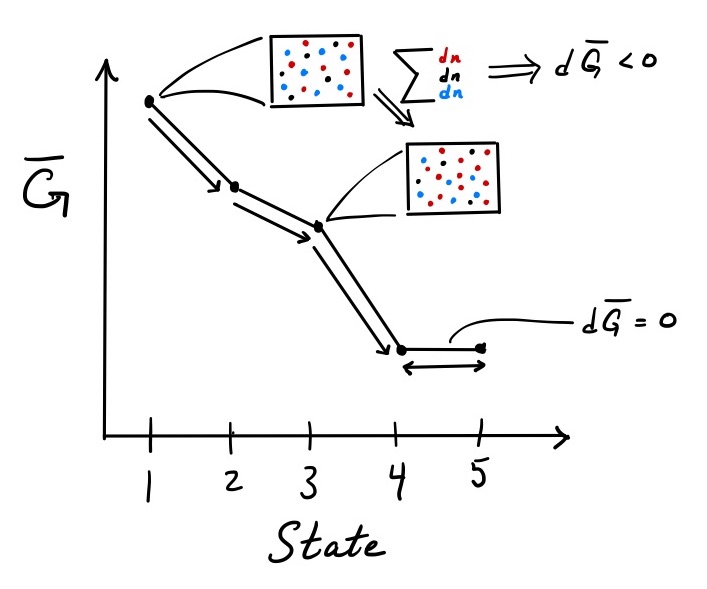
Figure 1: Dependence of Gibbs free energy of a system on chemical composition
Once the system reaches state 2, it cannot turn back. Doing so would require an increase in \(\overline{G}\) and contradicts Eq. \ref{eqcriteriaGbar}. In this fashion, the system will progress from states 2 to 3 to 4. Transitions \(1 \rightarrow 2 \rightarrow 3 \rightarrow 4\) are irreversible. And, as the system undergoes these changes due to reaction, the extensive Gibbs free energy of the system decreases.
The movement of the system down the Gibbs free energy curve continues until it reaches state 4. When the system shifts from state 4 to 5, \(d\overline{G} = 0\). The reverse step does the same and is therefore permissible. Transitions between states 4 and 5 are reversible. At the minimum of the Gibbs free energy landscape, the driving force for chemical change (\(d\overline{G} \le 0\)) has disappeared, and the system has reached its equilibrium.
7.4 Deriving the chemical equilibrium criteria
We have observed that equlibrium occurs when the Gibbs free energy of the system reaches a minimum where
\begin{equation} \sum_i{\hat{G}_i dn_i} = 0 \label{equilGi} \end{equation}
To find the minimum, we need a procedure to calculate \(\hat{G}_i\). As with all energy calculations, we begin by defining a reference point and tallying up the energy needed to get to the state-of-interest. In this case, for each species, we identify its elemental components and assign a value of 0 for their Gibbs free energy as pure elemental components at standard-state pressure (\(P^{o} = 1\) bar) and reaction temperature \(T\). From this reference, our first step is to assemble each molecular species \(i\) in pure form from its elemental parts at \(P^{o}\) and \(T\). The energy associated with this step is the molar standard-state Gibbs free energy of formation of species \(i\), \(\Delta G^o_{f,i}\). In the final step7, we take the molecular species at standard-state (pure component at \(P^o\)) to the state-of-interest in the reaction mixture at reaction \(P\). This final contribution to molar Gibbs free energy is modeled as \(RT \ln{\hat{a_i}}\) where \(\hat{a_i}\) is the activity of species \(i\). Assembling the contributions from each step, the molar Gibbs free energy of species in the reaction mixture is
\begin{equation} \hat{G}_i = \Delta G^o_{f,i} + RT \ln{\hat{a_i}} \label{calcGi} \end{equation}
where \(\hat{a_i} = \gamma_i C_i / C_i^o\) and \(C_i^o = 1\) M for liquid species \(i\). For gas species, the concentration \(C_i\) is replaced by the partial pressure \(p_i\) and the standard-state concentration is given by \(P^o\).
Incorporating \ref{calcGi} into \ref{equilGi}, we have
\begin{equation} \sum_i{\left( \Delta G^o_{f,i} + RT \ln{\hat{a_i}} \right) dn_i} = 0 \end{equation}
When a reaction occurs, the change in moles of species is directly related to the extent of reaction: \(dn_i = \nu_i d\xi\). Using this relationship and recognizing that the extent of reaction is the same for every species, we can rewrite the above as
\begin{equation} d\xi \sum_i{\left( \Delta G^o_{f,i} + RT \ln{\hat{a_i}} \right) \nu_i} = 0 \end{equation}
Eliminating \(d\xi\) and rearranging gives
\begin{align} \sum_i{\nu_i \Delta G^o_{f,i}} &= - RT \sum_i{ \nu_i \ln{\hat{a_i}}} \\ &= - RT \ln { \left( \prod_i{ \hat{a_i}^{\nu_i} } \right) } \end{align}
The left hand side is molar standard-state Gibbs free energy of reaction and the right hand side is the equilibrium constant:
\begin{equation} \Delta G^o_{R} = - RT \ln{K_a} \end{equation}
8 Simultaneous reactions in biological systems
Rarely in biology do we deal with an isolated reaction. Biological processes are typically mediated by networks of reactions. Metabolism, signal transduction, plasma coagulation and blood clotting and countless other examples remind us that dealing with multiple simultaneous reactions is the norm not the exception. It is therefore essential that we develop a systematic approach to deal with systems comprised of multiple reactions.
8.1 Example: Hemoglobin binding to oxygen
Tetrameric human hemoglobin can bind up to four oxygen molecules, one per subunit. The reactions describing the loading of oxygen onto hemoglobin are:
\begin{align} \begin{split} \ce{Hb0 + O2 & <=>[k_1][k_{-1}] Hb1} \\ \ce{Hb1 + O2 & <=>[k_2][k_{-2}] Hb2} \\ \ce{Hb2 + O2 & <=>[k_3][k_{-3}] Hb3} \\ \ce{Hb3 + O2 & <=>[k_4][k_{-4}] Hb4} \end{split} \label{rx:hemoglobin} \end{align}
where Hb\(_k\) denotes hemoglobin bound to \(k\) oxygen molecules.
Our goal is to model the dynamics of the reaction. That is, we seek a set of equations that, when solved using a clearly discernible procedure, will predict the amounts of each species over time.
Molecular species balance
Modeling the dynamics must account for the fact that oxygen can participate in multiple reactions. The amount of oxygen \(n_{\ce{O2}}\) is now affected by its consumption in all four forward reactions, each with its own extent of reaction. Thus, the molecular species balance on oxygen is:
\begin{equation} n_{\ce{O2}} = n_{\ce{O2}}^o + \nu_{\ce{O2},1}\xi_1 + \nu_{\ce{O2},2}\xi_2 + \nu_{\ce{O2},3}\xi_3 + \nu_{\ce{O2},4}\xi_4 \label{ox_spbal_long} \end{equation}
where \(\xi_j\) is the net reaction progress of reversible reaction \(j\). For each reversible reaction, the net reaction progress is the balance of forward and reverse reactions: \(\xi_j = \xi_{j,f} - \xi_{j,r}\). Note that all reactions \(j = 1…4\) are represented in \eqref{ox_spbal_long}.
To account for the moles of \(\ce{O2}\) consumed in each reaction, the net extent of each reaction is multiplied by the corresponding stoichiometric factor for oxygen in that reaction. Because oxygen is a reagent in every reaction, all stoichiometric factors are negative. Thus, \eqref{ox_spbal_long} becomes
\begin{equation} n_{\ce{O2}} = n_{\ce{O2}}^o - \xi_1 - \xi_2 - \xi_3 - \xi_4 \label{ox_spbal_short} \end{equation}
Similar species balances can be written for the hemoglobin species. For example, for \(\ce{Hb2}\), the molecular species balance is:
\begin{equation} n_{\ce{Hb2}} = n_{\ce{Hb2}}^o + \xi_2 - \xi_3 \label{Hb_spbal} \end{equation}
The species balances for \(\ce{Hb0}\) and \(\ce{Hb4}\) are a little different. Try to write them. See Eq. \eqref{spbalanceHbO2} for the solution.
Significance of molecular species balance
Molecular species balances provide a powerful piece of information. They tell us that the amounts of each species (\(n_i\)) are interdependent. The amounts of each species are coupled by their participation in a common set of reactions.
The challenge, however, is that untangling the coupling is difficult when multiple reactions are involved. For example, if \(n_{\ce{Hb2}}\) increases, what can we conclude about \(n_{\ce{O2}}\)? We might argue that oxygen amount must go down because \(\ce{Hb2}\) is produced by reaction of \(\ce{Hb1}\) with oxygen. Alternatively, one could argue oxygen amount must increase: \(\ce{Hb2}\) level will increase when oxygen dissociates from \(\ce{Hb3}\). Of course, the reality is that both processes are occuring simultaneously and whether oxygen amount increases or decreases will depend on the degree to which each reaction progresses.
Our goal is to utilize the molecular species balances in a systematic way to decipher the coupled dynamics of the reaction system. Tackling this problem generally breaks down into two steps, as described below.
Molecular species balances provides relationships between amounts of species
The first step is to find direct relationships between \(n_i\) by eliminating \(\xi_j\) from the molecular species balances. For example, we might find a direct relationship between \(n_{\ce{O2}}\) and \(n_{\ce{Hb2}}\) that resolves our debate above.
The species balances for this system are:
\begin{align} \begin{split} n_{\ce{Hb0}} &= n_{\ce{Hb0}}^o - \xi_1 \\ n_{\ce{Hb1}} &= n_{\ce{Hb1}}^o + \xi_1 - \xi_2 \\ n_{\ce{Hb2}} &= n_{\ce{Hb2}}^o + \xi_2 - \xi_3 \\ n_{\ce{Hb3}} &= n_{\ce{Hb3}}^o + \xi_3 - \xi_4 \\ n_{\ce{Hb4}} &= n_{\ce{Hb4}}^o + \xi_4 \\ n_{\ce{O2}} &= n_{\ce{O2}}^o - \xi_1 - \xi_2 - \xi_3 - \xi_4 \end{split} \label{spbalanceHbO2} \end{align}
Defining \(\Delta n_i \equiv n_i - n_i^o\) and rewriting as an augmented matrix, we obtain:
\begin{equation} \left[ \begin{array}{cccc|c} -1 & 0 & 0 & 0 & \Delta n_{\ce{Hb0}} \\ 1 & -1 & 0 & 0 & \Delta n_{\ce{Hb1}} \\ 0 & 1 & -1 & 0 & \Delta n_{\ce{Hb2}} \\ 0 & 0 & 1 & -1 & \Delta n_{\ce{Hb3}} \\ 0 & 0 & 0 & 1 & \Delta n_{\ce{Hb4}} \\ -1 & -1 & -1 & -1 & \Delta n_{\ce{O2}} \end{array} \right] \end{equation}
Gaussian elimination gives the row-reduced Echelon form:
\begin{equation} \left[ \begin{array}{cccc|c} 1 & 0 & 0 & 0 & - \Delta n_{\ce{Hb0}} \\ 0 & 1 & 0 & 0 & - \Delta n_{\ce{Hb0}} - \Delta n_{\ce{Hb1}} \\ 0 & 0 & 1 & 0 & - \Delta n_{\ce{Hb0}} - \Delta n_{\ce{Hb1}} - \Delta n_{\ce{Hb2}} \\ 0 & 0 & 0 & 1 & - \Delta n_{\ce{Hb0}} - \Delta n_{\ce{Hb1}} - \Delta n_{\ce{Hb2}} - \Delta n_{\ce{Hb3}} \\ 0 & 0 & 0 & 0 & - \Delta n_{\ce{Hb0}} - \Delta n_{\ce{Hb1}} - \Delta n_{\ce{Hb2}} - \Delta n_{\ce{Hb3}} -\Delta n_{\ce{Hb4}} \\ 0 & 0 & 0 & 0 & \Delta n_{\ce{O2}} - 4 \Delta n_{\ce{Hb0}} - 3 \Delta n_{\ce{Hb1}} - 2 \Delta n_{\ce{Hb2}} - \Delta n_{\ce{Hb3}} \end{array} \right] \label{rowReducedHbO2} \end{equation}
The last two rows give us relationships among the moles of each species:
\begin{align} \Delta n_{\ce{Hb4}} &= - \left( \Delta n_{\ce{Hb0}} + \Delta n_{\ce{Hb1}} + \Delta n_{\ce{Hb2}} + \Delta n_{\ce{Hb3}} \right) \label{conservHb} \\ \Delta n_{\ce{O2}} &= 4 \Delta n_{\ce{Hb0}} + 3 \Delta n_{\ce{Hb1}} + 2 \Delta n_{\ce{Hb2}} + \Delta n_{\ce{Hb3}} \label{conservO2} \end{align}
Eq. \eqref{conservHb} is a statement of conservation of hemoglobin, and Eq. \eqref{conservO2} accounts for conservation of oxygen. The former is intuitive, but the latter less so. The coefficients in Eq. \eqref{conservO2} are not immediately obvious but can be rationalized after some thought8. It underscores the benefit of the systematic procedure outlined here to derive the connections between amounts of species.
What about the first four rows of \eqref{rowReducedHbO2}? Each row relates an extent of reaction (\(\xi_j\)) to changes in moles of species. Since our goal is to model the time-evolution of amounts of species, we do not seek solutions for \(\xi_j\). However, we are interested in the time-derivative of \(\xi_j\) in the next step.
Rate laws
So far, we have not accounted for how the system evolves in time. To do so, we need to incorporate models for the rates of each reaction: \(d\xi_j/dt\). Thus, the second step is to take the time-derivative of the species balances \eqref{spbalanceHbO2}:
Taking the time-derivative of \ref{ox_spbal_short} shows that a model of the dynamics of oxygen concentration must account for all reactions in which oxygen participates:
\begin{align} \begin{split} \frac{dn_{\ce{O2}}}{dt} & = \nu_{\ce{O2},1} \frac{d\xi_1}{dt} + \nu_{\ce{O2},2} \frac{d \xi_2}{dt} + \nu_{\ce{O2},3} \frac{d \xi_3}{dt} + \nu_{\ce{O2},4} \frac{d \xi_4}{dt} \\ & = - \frac{d\xi_1}{dt} - \frac{d \xi_2}{dt} - \frac{d \xi_3}{dt} - \frac{d \xi_4}{dt} \end{split} \end{align}
where the rate of progress of each reaction is a balance of forward and reverse rates: each \(d\xi_j/dt = d\xi_{j,f}/dt - d\xi_{j,r}/dt\).
We can replace each \(d\xi_j/dt\) with an appropriate model for the rate law for reaction \(j\). If we assume reactions \eqref{rx:hemoglobin} are elementary, then we can apply the Law of Mass Action. For example, for reversible reaction 1, we write:
\begin{equation} \frac{1}{V_r} \frac{d \xi_1}{dt} = \frac{1}{V_r} \frac{d \xi_{1,f}}{dt} - \frac{1}{V_r} \frac{d \xi_{1,r}}{dt} = k_1 \ce{Hb0} \ce{O2} - k_{-1} \ce{Hb1} \end{equation}
Thus, the rate of change in oxygen concentration is modeled as:
\begin{align} \begin{split} \frac{1}{V_R} \frac{dn_{\ce{O2}}}{dt} = & - k_1 \ce{Hb0} \ce{O2} + k_{-1} \ce{Hb1} \\ & - k_2 \ce{Hb1} \ce{O2} + k_{-2} \ce{Hb2} \\ & - k_3 \ce{Hb2} \ce{O2} + k_{-3} \ce{Hb3} \\ & - k_4 \ce{Hb3} \ce{O2} + k_{-4} \ce{Hb4} \end{split} \end{align}
Because each reaction is reversible, two terms — a forward and backward rate — are used for each reaction. If a reaction is one-way, only one term would appear in the model.
Similar equations can be written for the rates of change in each hemoglobin species. For example, the rate of change in \(\ce{Hb2}\) is:
\begin{align} \begin{split} \frac{1}{V_R} \frac{dn_{\ce{Hb2}}}{dt} = &\ k_2 \ce{Hb1} \ce{O2} - k_{-2} \ce{Hb2} \\ & -k_3 \ce{Hb2} \ce{O2} + k_{-3} \ce{Hb3} \end{split} \end{align}
While it is straightforward to follow the procedure and write six rate equations, one for each species, it is prudent to pause and take stock of the situation.
The final dynamical model
The time-dependent variables in the system are the amounts of each species. For six species, six independent equations are required for a solvable model. The species balances (Eqs. \ref{conservHb} and \ref{conservO2}) already provide two. They tell us that the amounts of two species (e.g., \(\ce{Hb4}\) and \(\ce{O2}\)) can be calculated if we know the quantity of four remaining species — i.e., the amounts of these two species9 are determined fully and are not independent of the remaining four. Therefore, to specify fully the dynamical model for this system, we need only four rate equations, one for each of the remaining four remaining species: \(\ce{Hb0}\), \(\ce{Hb1}\), \(\ce{Hb2}\) and \(\ce{Hb3}\).
Altogether, the following six equations — two conservation equations and four rate equations — constitute our dynamical model:
\begin{equation} \frac{d\ce{Hb0}}{dt} = -k_1 \ce{Hb0} \ce{O2} + k_{-1} \ce{Hb1} \label{rateHb0} \end{equation}
\begin{align} \begin{split} \frac{d\ce{Hb1}}{dt} = &\ k_1 \ce{Hb0} \ce{O2} - k_{-1} \ce{Hb1} \\ & -k_2 \ce{Hb1} \ce{O2} + k_{-2} \ce{Hb2} \end{split} \end{align}
\begin{align} \begin{split} \frac{d\ce{Hb2}}{dt} = &\ k_2 \ce{Hb1} \ce{O2} - k_{-2} \ce{Hb2} \\ & -k_3 \ce{Hb2} \ce{O2} + k_{-3} \ce{Hb3} \end{split} \end{align}
\begin{align} \begin{split} \frac{d\ce{Hb3}}{dt} = &\ k_3 \ce{Hb2} \ce{O2} - k_{-3} \ce{Hb3} \\ & -k_4 \ce{Hb3} \ce{O2} + k_{-4} \ce{Hb4} \end{split} \label{rateHb3} \end{align}
\begin{align} \Delta \ce{Hb4} &= - \left( \Delta \ce{Hb0} + \Delta \ce{Hb1} + \Delta \ce{Hb2} + \Delta \ce{Hb3} \label{conservHb_2} \right) \\ \Delta \ce{O2} &= 4 \Delta \ce{Hb0} + 3 \Delta \ce{Hb1} + 2 \Delta \ce{Hb2} + \Delta \ce{Hb3} \label{conservO2_2} \end{align}
where we have assumed constant volume.
The model is solved by using Eqs. \ref{conservHb_2} and \ref{conservO2_2} to replace all occurrences of \(\ce{Hb4}\) and \(\ce{O2}\) in differential equations \ref{rateHb0} - \ref{rateHb3} with \(\ce{Hb0}\), \(\ce{Hb1}\), \(\ce{Hb2}\) and \(\ce{Hb3}\). The system of four differential equations are then solved numerically. The solutions obtained for \(\ce{Hb0}\), \(\ce{Hb1}\), \(\ce{Hb2}\) and \(\ce{Hb3}\) are then applied in algebraic equations \ref{conservHb_2} and \ref{conservO2_2} to determine \(\ce{Hb4}\) and \(\ce{O2}\).
9 Sequential reactions and yield
Sequential reaction pathways are a common reaction motif in biological systems. A simple example composed of elementary reactions is:
\begin{equation} \ce{A -> B -> C} \label{rx:sequential} \end{equation}
9.1 Maximizing yield as an engineering objective
In an engineering context, if the objective is to produce B — e.g., a biofuel or pharmaceutical — using host cells as ``factories", we are interested in determining the optimal time to halt the reaction and extract B. If we extract too soon, we expect that there may not have been sufficient conversion of A into B. If we extract too late, we may lose too much B to downstream production of C.
The goal of producing as much B for every mole of A supplied can be framed in terms of maximizing the yield of B (\(Y_B\)). The yield is defined here as the amount of B produced relative to the theoretical maximum that could be produced. In this case, the theoretical or idealized maximum occurs if every mole of A supplied were converted into B and none into C. That is,
\begin{equation} Y_B = \frac{n_B - n_B^o}{n_A^o} \end{equation}
The yield has a minimum value of 0, and at best, its value attains the theoretical maximum of 1.
With this metric for yield, we can attempt to predict the maximum yield given a sequential reaction system such as \eqref{rx:sequential}. At what time is yield maximized? To begin to answer these and other questions, we need to develop a model of the dynamics of the system of reactions.
9.2 Modeling sequential reactions
Molecular species balance
We begin by writing the molecular species balances for each species. The number of moles of each species is equal to the amount at the beginning plus any moles generated — and minus any that is consumed — by reactions in which the species participates. For \eqref{rx:sequential}, the molecular species balances are:
\begin{alignat}{2} \begin{split} n_A & = n_A^o - \xi_1 \\ n_B & = n_B^o + \xi_1 & - \xi_2 \\ n_C & = n_C^o & + \xi_2 \end{split} \label{sequentialSpBal} \end{alignat}
The above can be rewritten as an augmented matrix:
\begin{equation} \left[ \begin{array}{cc|c} -1 & 0 & \Delta n_A \\ 1 & -1 & \Delta n_B \\ 0 & 1 & \Delta n_C \end{array} \right] \end{equation}
where \(\Delta n_i = n_i - n_i^o\). Gaussian elimination gives the row-reduced Echelon form:
\begin{equation} \left[ \begin{array}{cc|c} 1 & 0 & - \Delta n_A \\ 0 & 1 & \Delta n_C \\ 0 & 0 & \Delta n_A + \Delta n_B + \Delta n_C \end{array} \right] \end{equation}
Reading from the final row, we find that:
\begin{equation} n_A + n_B + n_C = n_A^o + n_B^o + n_C^o \end{equation}
which simplifies to
\begin{equation} A + B + C = A_o + B_o + C_o \label{spbal_sequential} \end{equation}
for a constant-volume reaction. The concentrations of A, B and C present at any specific time must be equal to the total initial concentrations of species for a constant-volume system. Equation \ref{spbal_sequential} is a statement of conservation, and for this simple system, it could have been written based on intuition. However, the systematic approach of writing out molecular species balances and using Gaussian elimination to determine direct relationships between amounts of species is useful in more complex reaction systems.
From the perspective of developing a dynamical model, Eq. \eqref{spbal_sequential} serves a practical purpose. If we were to find the solution to \(A(t)\) and \(B(t)\), Eq. \eqref{spbal_sequential} gives us \(C(t)\) with little effort.
Rate equations
To obtain the dynamics of \(A\) and \(B\), we turn to the rates at which reactions occur. Taking the time-derivative of Eq. \eqref{sequentialSpBal}, we see that
\begin{alignat*}{2} \begin{split} \dot{n}_A & = - \dot{\xi}_1 \\ \dot{n}_B & = - \dot{\xi}_1 & - \dot{\xi}_2 \\ \dot{n}_C & = & + \dot{\xi}_2 \end{split} \end{alignat*}
where Newton’s notation is used for time-derivatives. Using the Law of Mass Action to model elementary reactions \eqref{rx:sequential}, we write:
\begin{align} \dot{n}_A & = -k_1 A V_R \\ \dot{n}_B & = k_1 A V_R - k_2 B V_R \\ \dot{n}_C & = k_2 B V_R \end{align}
Assuming constant volume,
\begin{align} \dot{A} & = -k_1 A \label{dAdt_sequential} \\ \dot{B} & = k_1 A - k_2 B \label{dBdt_sequential} \\ \dot{C} & = k_2 B \label{dCdt_sequential} \end{align}
The dynamical model and its solution
Since the system consists of three variables, we will use one species balance \eqref{spbal_sequential} together with two of the three rate equations (Eqs. \ref{dAdt_sequential}, \ref{dBdt_sequential}) to model the system.
Using \eqref{dAdt_sequential}, we find that
\begin{equation} A = A_o e^{-k_1 t} \label{solnA_sequential} \end{equation}
where \(A_o\) is the initial concentration of A. Putting \eqref{solnA_sequential} in \eqref{dBdt_sequential} gives
\begin{equation} \frac{dB}{dt} + k_2 B = k_1 A_o e^{-k_1 t} \end{equation}
This differential equation is linear with non-constant coefficients and can be solved using an integration factor \(\rho(t) = e^{\int{k_2 dt}}\). The solution is given by
\begin{align} \int_0^t{d(\rho B)} = \int_0^t{\rho k_1 A_o e^{-k_1 t} dt} \end{align}
With an intial condition of \(B_o = 0\), the solution is
\begin{equation} B = \frac{k_1 A_o}{k_2-k_1} \left( e^{-k_1t} - e^{-k_2t} \right) \label{solnB_sequential} \end{equation}
Finally, with an initial condition of \(C_o = 0\), we use the species balance \eqref{spbal_sequential} and our solutions for A \eqref{solnA_sequential} and B \eqref{solnB_sequential} to obtain C:
\begin{align} \begin{split} C & = A_o + B_o + C_o - A - B \\ & = A_o - A - B \\ & = A_o \left( 1 - e^{-k_1t} - \frac{k_1}{k_2-k_1} \left( e^{-k_1t} - e^{-k_2t} \right) \right) \end{split} \end{align}
10 Competing reactions
In a system with two competing reactions, a reagent is consumed via separate pathways. A simple schematic consisting of two first-order elementary reactions is the following:
\begin{equation} \begin{split} \ce{A ->[k_1] B} \\ \ce{A ->[k_2] C} \end{split} \label{rx:competing} \end{equation}
Two different products (B and C) are formed. A common engineering challenge is to maximize production of a preferred product, say B, relative to unwanted side-products. We define a metric, selectivity, to help guide and evaluate design options.
10.1 Defining selectivity
Depending on design goals, different definitions of selectivity may be used.
Fractional selectivity
One metric is fractional selectivity (\(S_f^B\)). It is the extent of progress of the reaction (\(\xi_1\)) producing desired species B normalized to the total extent of reaction progress along all pathways that consume A (\(\xi_1 + \xi_2\)). For the simple competing reaction scheme \eqref{rx:competing}, fractional selectivity in producing B is:
\begin{align} \begin{split} S_f^B & = \frac{\xi_1}{\xi_1 + \xi_2} \\ & = \frac{n_B - n_B^o}{(n_B-n_B^o) + (n_C - n_C^o)} \end{split} \label{frac_selectivity} \end{align}
Relative selectivity
Another metric is relative selectivity (\(S_r^B\)), the ratio of the extent of reaction producing B to the extent of reaction producing C:
\begin{equation} S_r^B = \frac{\xi_1}{\xi_2} = \frac{n_B - n_B^o}{n_C-n_C^o} \end{equation}
Comparisons
Fractional selectivity is bound between 0 and 1 for the simple competing reaction \eqref{rx:competing}, whereas relative selectivity is not.
Furthermore, both definitions above were stated in terms of extents of reaction (\(\xi_1\) and \(\xi_2\)). An alternative is to define them in terms of moles of species produced (\(n_b - n_b^o\) and \(n_c - n_c^o\)). The former normalizes for stoichiometric coefficients. Precisely which definition is used should be stated clearly and kept consistent. When comparing reported selectivity values, it is recommended to be aware of the definition being used.
The need for a dynamical model
To determine how selectivity depends on parameters, such as \(k_1\) and \(k_2\), of the reaction system, we need to develop a predictive model of the competing reactions \eqref{rx:competing}.
10.2 Molecular species balances
We begin by writing molecular species balances, with one balance for each species in the system. For a closed system, we know that the amount of each molecular species at any given time must be equal to the amount with which we started, adjusted for any consumption or production of that species. For the amount of species A, for example, we can write:
\begin{equation} n_A = n_A^o - \xi_1 - \xi_2 \end{equation}
where \(n_A\) and \(n_A^o\) are the moles of at A at time \(t\) and at initial time, respectively, and \(\xi_j\) are the extents to which reactions 1 and 2 have proceeded. If volume is constant, the species balance can be written in terms of concentration, as follows:
\begin{equation} A = A_o - \xi_1^* -\xi_2^* \end{equation}
where the asterisk denotes extents of reaction per unit volume. Altogether, we can write three species balances for this system:
\begin{alignat*}{1} %\begin{split} A & = A_o - & \xi_1^* & -\xi_2^* \\ B & = B_o + & \xi_1^* \\ C & = C_o & & + \xi_2^* %\end{split} \end{alignat*}
With two reactions in the system, only two of these three species balances are needed to specify the progress of the two reactions. The third equation will provide an additional constraint — a relationship among A, B and C — that is independent of the extents of reactions. To identify this relationship, we write the system of reactions in matrix form, treating \(\xi_j\) as variables, and bring the matrix to reduced-row echelon form, as shown below:
\begin{equation} \left[ \begin{array}{cc|c} -1 & -1 & A-A_o \\ 1 & 0 & B-B_o \\ 0 & 1 & C-C_o \\ \end{array} \right] \rightarrow \left[ \begin{array}{cc|c} 1 & 0 & \Delta B \\ 0 & 1 & \Delta C \\ -1 & -1 & \Delta A \\ \end{array} \right] \rightarrow \left[ \begin{array}{cc|c} 1 & 0 & \Delta B \\ 0 & 1 & \Delta C \\ 0 & 0 & \Delta A + \Delta B + \Delta C \\ \end{array} \right] \end{equation}
where \(\Delta X = X - X_o\) for each species \(X\). From the final row, we derive an important constraint on the closed sytem:
\begin{equation} A + B + C = A_o + B_o + C_o \label{spbal_competing} \end{equation}
This molar species balance tells us that the total moles of A, B and C at any given time must be equal to the total moles of A, B and C with which the reaction begins for this system. It is critical to underscore that this molar balance is not a general conservation rule! Moles of species are not conserved.
10.3 Law of Mass Action provides a framework to model system dynamics
A quick tabulation of the number of unknown variables (three — A, B, C) and the number of equations (one species balance) reveals that we need two more equations to model the system. We turn to relationships that specify how the system variables will evolve in time. Because \eqref{rx:competing} are elementary reactions, we use the Law of Mass Action to write a system of differential equations for the rates of change in the concentration of each species:
\begin{align} \frac{dA}{dt} & = - k_1 A - k_2 A \label{dAdt_competing}\\ \frac{dB}{dt} & = k_1 A \label{dBdt_competing} \\ \frac{dC}{dt} & = k_2 A \label{dCdt_competing} \end{align}
Only two of the three differential equations are independent, as we already have a relationship relating A, B and C through \eqref{spbal_competing}.
Equation \eqref{dAdt_competing} that models the rate of change in A is appealing because it is a readily-solvable differential equation with a single variable. The solution is:
\begin{equation} A = A_o e^{-(k_1+k_2)t} \label{solnA_competing} \end{equation}
We can then use \eqref{solnA_competing} in \eqref{dBdt_competing}, yielding
\begin{equation} \frac{dB}{dt} = k_1 A_o e^{-(k_1+k_2)t} \end{equation}
Solving this differential equation by separating the variables gives:
\begin{equation} B = B_o +\frac{k_1}{k_1+k_2} A_o (1-e^{-(k_1+k_2)t}) \label{solnB_competing} \end{equation}
Finally, we obtain C using \eqref{spbal_competing} without the need for \ref{dCdt_competing}:
\begin{align} \begin{split} C & = A_o + B_o + C_o - A - B \\ & = C_o + \frac{k_2}{k_1+k_2} A_o (1-e^{-(k_1+k_2)t}) \end{split} \label{solnC_competing} \end{align}
10.4 Selectivity in producing B is related to ratio of rate constants for competing pathways
Having derived the time-evolution of each species, the fractional selectivity in producing B is given by \eqref{frac_selectivity}. For this system, it is
\begin{equation} S_f^B = k_1/(k_1 + k_2) \end{equation}
Thus, conditions that increase \(k_1\) relative to \(k_2\) provide an avenue for selectively producing B.
11 Reversible binding reaction
We dealt with reversible reactions when we discussed equilibrium. We determined how to find the point of equilibrium. Here, we want to consider the dynamics. How do concentrations of species change in time as the system moves toward equilibrium?
Consider the following elementary equilibrium reaction:
\begin{equation} \ce{ A + B <=>[k_f][k_r] C} \end{equation}
We write the molecular species balance, accounting for how each species in the reaction is consumed and generated through reactions:
\begin{alignat*}{3} n_A & = n_A^o & - \xi_f & + \xi_r \\ n_B & = n_B^o & - \xi_f & + \xi_r \\ n_C & = n_C^o & + \xi_f & - \xi_r \end{alignat*}
where the extents of forward (\(\xi_f\)) and reverse (\(\xi_r\)) reaction appear always as a difference. We can substitute a net extent of forward reaction (\(\xi\)) for \(\xi_f - \xi_r\) and write the species balances as:
\begin{alignat*}{3} n_A & = n_A^o & - \xi \\ n_B & = n_B^o & - \xi \\ n_C & = n_C^o & + \xi \end{alignat*}
Eliminating \(\xi\) from these equations and assuming volume is constant, we identify two molar species balances:
\begin{align} A - A_o & = - (C - C_o) \\ B - B_o & = - (C - C_o) \label{eq:revrxn-speciesbalance} \end{align}
Using \eqref{eq:revrxn-speciesbalance}, the dynamics of A and B can be readily determined once we know the dynamics of C. Thus, we need only rate equation for C to solve the dynamics of this system. For a constant-volume reaction, the rate of change in the concentration of C is given by:
\begin{align} \frac{dC}{dt} & = k_f A B - k_r C \\ & = k_f (A_o-(C-C_o)) (B_o-(C-C_o)) - k_r C \label{eq:revrxn-ratelaw} \end{align}
Solving Eq. \eqref{eq:revrxn-ratelaw} will give the dynamics of C. We can then find \(A(t)\) and \(B(t)\) using \eqref{eq:revrxn-speciesbalance}. While the strategy for solving the dynamics of this reaction system is clear, the differential equation in \eqref{eq:revrxn-ratelaw} is non-linear, suggesting that even relatively simple-looking reaction systems can lead to seemingly challenging equations. We would like to gain insights into the dynamics of such nonlinear systems without having to rely upon complex analytical integration or computational methods.
12 Graphical analysis of a non-linear first-order system
Phase portrait analysis is a powerful graphical method for gaining significant insights into the dynamical behavior of a system without integration of model equations.
Here, we will apply phase portrait analysis to our model of a reversible reaction. The model consists of a first-order differential equation given by:
\begin{equation} \frac{dC}{dt} = f( C) = k_f (A_o + C_o -C) (B_o+C_o - C) - k_r C \label{eq:revrxn_phaseportrait} \end{equation}
Phase portrait analysis begins with plotting \(f( C)\) (Figure 2). That is, construct a plot with \(dC/dt\) on the y-axis and the system variable \(C\) on the x-axis. Since we do not have numerical values for the rate constants and initial amounts of species, we approach the plot from an analysis of \(f( C)\) and use physical arguments to constrain the domain of \(C\). Using this approach, we can make the following conclusions about the phase portrait:
-
Since the \(C^2\) term in \(f( C)\) has a positive coefficient, the plot is a concave-up parabola.
-
The physically-relevant domain for this system is \(0 \le C \le C_o + \mathrm{min}\{A_o,B_o\}\). That is, even if the reaction proceeded completely toward products, \(C\) can at most be the original concentration \(C_o\) plus the concentration of the limiting reagent.
-
The y-intercept is \(f(C=0) = k_f (A_o+C_o)(B_o+C_o)\).
-
The minimum in \(f( C)\) occurs beyond the maximum physically-relevant value for \(C\). The value \(C^*\) at which \(f( C)\) is a minimum is found readily by setting \(df/dC = 0\).
\begin{align} f'(C^*) & = 2 k_f C^* - (A_o+B_o+2C_o) k_f - k_r = 0 \\ \nonumber C^* & = \frac{k_r + (A_o+B_o+2C_o) k_f}{2 k_f} = \frac{k_r}{2k_f} + C_o + \frac{A_o+B_o}{2} \nonumber \end{align}
Because the average of two numbers, \(A_o\) and \(B_o\), is always greater than the smaller number, we see that \(C^* > C_o + \mathrm{min}\{A_o,B_o\}\). In the event \(A_o = B_o\), note that the rate constants are positive numbers and \(k_r/2k_f > 0\).
Taken together, this information leads us to a phase portrait with a clearly-defined, physically-relevant domain.
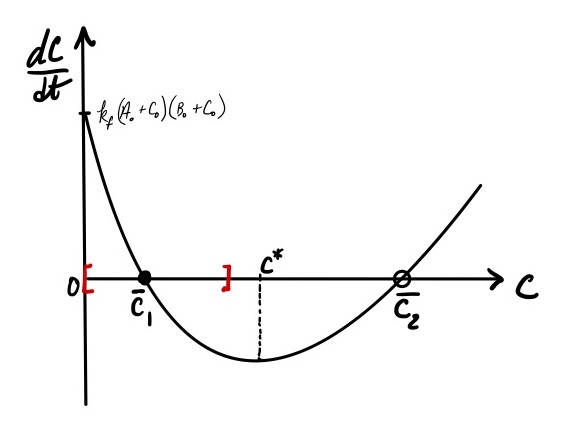
Figure 2: The phase portrait for the dynamics of a reversible reaction. The model is given by Eq. eqref{eq:revrxn_phaseportrait}. The red square brackets denote the physically relevant domain for the system. The stable ((overline{C}_1)) and unstable ((overline{C}_2)) fixed points are denoted by solid and empty circles on the x-axis. The point at which the rate of change in (C) is at a minimum is (C^*).
12.1 Fixed points and stability
The plot shows that a single root, \(C=\overline{C}_1\), lies in the physically-relevant domain. At this point, \(dC/dt = 0\), indicating that \(\overline{C}_1\) is a steady-state or fixed point of the system. A fixed point is locally stable if a slight perturbation in the value of C from its steady-state returns the system back to the steady-state. In this case, if the value of C is increased slightly above \(\overline{C}_1\), the value of \(dC/dt\) is negative, meaning the value of \(C\) will decrease and return the system toward the steady-state. Similarly, suppose the system were nudged to a slightly lower value of \(C\) from its steady-state \(\overline{C}_1\). Now, \(dC/dt\) has a positive value and \(C\) will increase, moving the system back toward the fixed point. Thus, when the system is perturbed locally to a slightly higher or lower value of C, it returns to the stable fixed point.
Although non-physical, it is worthwhile to consider briefly the other root \(C=\overline{C}_2\). This is a second steady-state or fixed point. Notice, however, that slightly perturbing the system away from this fixed point will cause the system to be repelled further from the steady-state. For example, a slight increase in \(C\) from \(\overline{C}_2\) leads to a positive \(dC/dt\), meaning that \(C\) will again increase. Thus, the system is propelled away from the fixed point. This fixed point is an unstable steady-state.
12.2 Predicting dynamics starting from an initial condition
The phase portrait not only identifies steady-states, but also can be used to predict the dynamical behavior of a system. The question we wish to explore is: how does the concentration of C evolve over time starting from a given initial condition? That is, produce a plot of \(C\) vs. \(t\) solely by using the phase portrait.
We will consider two cases with different initial conditions. In case (a), the initial concentration \(C_o = C_a\) where \(C_a < \overline{C}_1\). In case (b), \(C_o = C_b\) where \(C_b > \overline{C}_1\). Changing the value of \(C_o\) will change the model equation \eqref{eq:revrxn_phaseportrait} and the curve on Figure 2. To avoid this complication, when changing the value of \(C_o\) between the two cases, we assume that \(A_o\) and \(B_o\) are also changed such that \(X_o = A_o + C_o\) and \(Y_o = B_o + C_o\) are held constant. By holding \(X_o\) and \(Y_o\) constant between cases (a) and (b), the model equation is unchanged between the two cases, and the same phase portrait can be used to investigate the dynamical response of the system.
Case (a). From the phase portrait (Figure 3), it is evident that at \(t=0\) and \(C=C_a\), \(dC/dt > 0\). Thus, the concentration of C will increase at \(t=0\), and we can draw a segment with an upward-oriented slope on the time-course at this time point. Going back to the phase portrait, the system is now at a slightly higher \(C > C_a\). Here too, \(dC/dt\) remains positive but lower than when \(C=C_a\). Thus, we return to the time-course and draw a segment with a slightly lower upward slope. Repeating this process where we iterate between the phase portrait and the time-course, we see that the line segments on the time-course get progressively shallower with each advance in time as C progressively approaches \(\overline{C}_1\) in the phase portrait. When the system eventually arrives at \(\overline{C}_1\), the value of \(dC/dt\) reaches 0. At this point, the line segment on the time-course is flat. No further changes in \(C\) occur, and the system lands, as we expected, at its steady-state. Connecting the line segments on the time-course, we arrive at a semi-quantitative prediction for the dynamics of the system. The concentration of C begins at \(C_a\) and increases monotonically to a plateau at \(\overline{C}_1\). The rate at which the concentration increases steadily decreases, meaning there are no inflection points in the predicted behavior. Furthermore, there is no overshoot: the concentration does not increase past \(\overline{C}_1\) and return back.
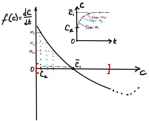
Figure 3: Predicting time-course (inset) from the phase portrait with the initial condition (C_o = C_a). For a particular value of (C) on the x-axis of the phase portrait, the value of (dC/dt) on the y-axis provides the slope ((m)) of the line segment drawn on the time-course (inset). Progressive iterations between the phase portrait and time-course are indicated by a color sequence: black to blue to red.
Case (b). Now, the initial condition is \(C_o = C_b\) (Figure 4). Consulting the phase portrait, \(dC/dt < 0\) at \(C_b\). Thus, we draw a downward-pointing line segment on the time-course at \(t=0\) where \(C=C_b\). The line segment projects that \(C\) decreases to a new value less than \(C_b\) at the next time point. We return to the phase portrait to determine the value of \(dC/dt\) at the new, lower \(C\). While the value of \(dC/dt\) remians negative, its absolute value decreases. With this information, we draw a new downward-pointing segment in the time-course, taking care to reduce the magnitude of the slope. Repeating this process, we graphically march forward in time on the time-course plot while consulting the phase portrait at each time step. Eventually, \(C\) approaches the fixed point \(\overline{C}_1\) where \(dC/dt = 0\). The system has reached steady-state.
To summarize, predicting the dynamical behavior of a system from its phase portrait is an iterative approach. We use the phase portrait to determine the rate of change in C at a known concentration of C. In the first iteration, the known concentration is the initial condition. We next use what we have learned about the rate of change in C to draw an appropriately-oriented line segment on the time course. This segment informs us whether the value of \(C\) increases or decreases. Now, with an updated value for \(C\), we return to the phase portrait to determine the rate of change in \(C\) at the new value of \(C\).
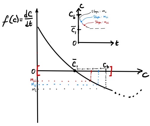
Figure 4: Predicting time-course (inset) from the phase portrait with the initial condition (C_o = C_b). See legend to Figure 3 for additional details.
12.3 Exploring a non-physical regime
In the two cases above, the dynamical behavior of \(C\) is to increase (or decrease) at a progressively lower rate until reaching a steady-state value of \(\overline{C}_1\). Since we established that the first-order model is physically relevant only in a domain where the concentration of C is less than the minimum of \(f( C)\), the dynamical behaviors we have seen are the only ones relevant to this physical system.
It is, however, worthwhile to explore theoretically other points on the phase portrait. The value in this exploration is that our observations could be relevant to other systems we encounter, even if it is not physically relevant to this system. For example, we have already seen the occurrence of an unstable steady-state at \(\overline{C}_2\).
Now, consider a theoretical condition in which the initial value of \(C_o\) is \(C^\dagger\) (Figure 5). The phase portrait tells us that because \(dC/dt < 0\), the system variable \(C\) must decrease in value over time. Note that the magnitude of \(dC/dt\) increases as the system moves initially to the left along the x-axis of the phase portrait. Thus, \(C\) is predicted to decrease progressively faster at the initial stages.
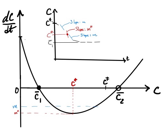
Figure 5: Predicting time-course (inset) from the phase portrait with the initial condition (C_o = C^dagger). See legend to Figure 3 for additional details.
Something interesting happens when the system reaches the minimum on the phase portrait. While \(dC/dt\) remains negative, its magnitude begins to decrease for each subsequent step in time. Thus, the value of \(C\) continues to decrease, but now, the rate at which \(C\) decreases gets progressively slower. This behavior continues as \(C\) ultimately approaches its steady-state value of \(\overline{C}_1\).
Taken together, a time-course of \(C\) shows an inflection point where the rate of decrease goes from progressively increasing to progressively decreasing. This inflection occurs at the value of \(C\) at which the phase portrait shows a minimum. Thus, a minimum (or maximum) in a phase portrait corresponds to a point of inflection on a time-course.
13 Simple receptor-ligand binding
Non-covalent interaction between a receptor and ligand to form a complex is pervasive in biological systems. A common scenario involves a receptor (R) on the surface of a cell that binds to a ligand (L) in the surrounding extracellular medium. The binding event forms a receptor-ligand complex (C), and unbinding dissociates the complex back to free receptor and ligand. The elementary reversible reaction is written as:
\begin{equation} \ce{R + L <=> C} \label{rx:simpleRL} \end{equation}
Suppose this receptor-ligand interaction is occurring among a population of \(n\) cells situated in a medium of volume \(V\)10. Each cell expresses \(R_T\) receptors, and the total concentration of ligand is \(L_o\).
We can model the dynamics of receptor-ligand binding by first writing species balances on receptors and ligands. The total number of receptors on a cell must exist either as free receptor of as a complex in a ligand-bound form:
\begin{equation} R_T = R + C \label{eq:Rbalance} \end{equation}
Note that the units on each term are # of molecules per cell.
Similarly, all ligand in the system must be found as either free ligand or receptor-bound ligand:
\begin{equation} N_{Av}VL_o = N_{Av}V L + n C \nonumber \end{equation}
where Avogadro’s number (\(N_{Av}\)) and \(V\) convert ligand concentration (\(L_o\) and \(L\)) to number of molecules and \(n C\) gives the total number of complexes in the system. Rearranging gives:
\begin{equation} L_o = L + \left(\frac{n}{N_{Av}V}\right) C \label{eq:Lbalance} \end{equation}
The species balances on receptor \eqref{eq:Rbalance} and ligand \eqref{eq:Lbalance} provide two constraints for a system with three time-dependent variables (R, L and C). The third and final relationship needed to solve the dynamics of the system captures the rate at which the system evolves in time.
Because \eqref{rx:simpleRL} is an elementary reaction, we model the rate of reaction using the Law of Mass Action to write:
\begin{equation} \frac{dC}{dt} = k_f RL - k_r C \nonumber \end{equation}
Substituting \(R\) and \(L\) with \(C\) using equations \eqref{eq:Rbalance} and \eqref{eq:Lbalance} gives:
\begin{equation} \frac{dC}{dt} = k_f (R_T-C)\left(L_o - \frac{n}{N_{Av}V} C \right) - k_r C \label{eq:RLdynamics} \end{equation}
The first-order non-linear model \eqref{eq:RLdynamics} has an analytical solution that can be written in implicit form, as detailed in Lauffenburger & Linderman, 1993. Here, we will take a different approach. We will gain insights into the solution for \(C(t)\) using a graphical approach without actually solving the differential equation. This approach is based on phase-plane analysis. Before embarking on this graphical approach, we first will recast \eqref{eq:RLdynamics} in a non-dimensional form.
13.1 Dimensional analysis
An informative first-step in analyzing the behavior of a model is to scale its dimensional variables into non-dimensional form. Rescaling adjusts a variable relative to a representative or characteristic value. For example, the number of complexes per cell (\(C\)) will range between 0 and R_T. Thus, we define a new variable \(u\) as
\begin{equation} u = C/R_T \label{dimlessC} \end{equation}
This definition rescales the number of complexes relative to a characteristic value, the total number of receptors per cell. The normalized measure of complexes (\(u\)) has at least two advantages. First, its range is [0, 1], providing a well-bounded metric of complex formation. Second, \(u\) has a simple physical interpretation. It is the fraction of receptors that are bound to ligand.
To scale time \(t\), we select a representative value for this system that carries units of time. The first-order rate constant, \(k_r\), is the most apparent choice, as its units are inverse time. Thus, we define a dimensionless time \(\tau\) as
\begin{equation} \tau = t/(1/k_r) \label{dimlessTime} \end{equation}
Next, we substitute our definitions \eqref{dimlessC} - \eqref{dimlessTime} into our model equation as follows
\begin{align} \frac{dC}{dt} & = k_f (R_T-C)\left(L_o - \frac{n}{N_{Av}V} C \right) - k_r C \nonumber \\ \frac{d(uR_T)}{d(\tau/k_r)} & = k_f (R_T-uR_T)\left(L_o - \frac{n}{N_{Av}V} uR_T \right) - k_r uR_T \nonumber \\ \frac{R_T}{1/k_r}\frac{du}{d\tau} & = k_f L_o R_T (1-u)\left(1 - \frac{n R_T}{N_{Av}VL_o} u \right) - k_r uR_T \nonumber \\ \end{align}
to obtain:
\begin{equation} \frac{du}{d\tau} = \frac{L_o}{K_d} (1-u)(1-\eta u) - u \label{eq:dimlessRLdynamics} \end{equation}
where \(\eta = n R_T / N_{Av} V L_o\). Note that all dimensional variables (\(C\) and \(t\)) are now replaced with dimensionaless counterparts (\(u\) and \(\tau\), respectively).
Two parameter groups emerge: \(L_o/K_d\) and \(\eta\). Both are dimensionless. And, both have clearly identifiable physical significance.
The first compares the concentration of ligand to the equilibrium dissociation constant. The physical significance of this dimensionless parameter is clear upon considering that \(K_d = L_o \overline{R} / \overline{C}\) where the bar denotes equilibrium. Thus, the higher the ligand concentration relative to \(K_d\), the higher the ratio of complexes to free receptors at equilibrium. That is, at higher \(L_o/K_d\), more receptors will be occupied with ligand.
The second dimensionless paramter \(\eta = n R_T / N_{Av} V L_o\) is a ratio of the number of receptors in the system (\(n R_T\)) to the number of ligands in the system (\(N_{Av} V L_o\)). When \(\eta «1\), ligand is significantly in excess of receptor. In this scenario, even when all receptors are bound to ligand, the amount of free ligand will remain approximately equal to the total initial amount of ligand. Binding does not deplete the amount of available, free ligand: \(L \approx L_o\).
On the other hand, when \(\eta > 1\), receptors outnumber ligand. Thus, it is impossible for all receptors on the cell surface to be occupied by ligand. The maximum number of receptors per cell that could be occupied when ligand is a limiting reagent is \(L_o N_{Av} V / n\).
Only two non-dimensional parameters (\(\eta\) and \(L_o/K_d\)) are needed to specify the quantitative dynamics of the scaled system. Compare this to the original dimensional system whose dynamics relied on values for a larger cast of parameters, \(k_f\), \(k_r\), \(L_o\), \(n\) and \(R_T\). We have reduced the parameter space from five for the dimensional model to just two for the non-dimensional model.
14 Predicting the dynamics of simple receptor-ligand binding
Dimensional analysis informs us that to understand the dynamics of receptor-ligand binding, we need only consider its dependence on two non-dimensional parameters, \(L_o/K_d\) and \(\eta = n R_T / N_{Av}V L_o\).
14.1 Ligand in excess (\(\eta « 1\))
We begin with the simpler scenario. Suppose ligand is supplied in excess of receptor. That is, the total concentraion of ligand is much greater than the concentration of receptors, \(L_o » n R_T / N_{Av} V\) or \(\eta « 1\). In this case, the non-linear model equation
\begin{equation} \frac{du}{d\tau} = \frac{L_o}{K_d} (1-u)(1-\eta u) - u \label{modelLdepletion} \end{equation}
reduces to
\begin{equation} \frac{du}{d\tau} = \frac{L_o}{K_d} (1-u) - u \label{modelLexcess} \end{equation}
At steady state11, we set \(du/d\tau = 0\) in Eq. \eqref{modelLexcess} and find
\begin{equation} \overline{u} = \frac{L_o}{L_o+K_d} \label{ssLexcess} \end{equation}
where \(\overline{u}\) denotes steady state.
The steady-state solution offers a useful heuristic. When the ligand concentration is equal to the dissociation constant (\(L_o = K_d\)), half of the cell surface receptors are bound to ligand (\(\overline{u} = 0.5\)). This rule-of-thumb can be handy when choosing a ligand concentration for treating cells or when interpreting a measured ligand concentration in a tissue in vivo. By comparing the applied or measured ligand concentration to \(K_d\), one gains an approximate gauge of fractional occupancy of cell surface receptors. Of course, this heuristic is valuable only when ligand is in excess. We turn to the other situation in the next subsection.
Like the steady-state solution, the dynamics of \(u\) is obtained easily when \(\eta «1\). The variables in Eq. \eqref{modelLexcess} are separable, and integration with initial condition \(u(0)=0\) leads to the solution:
\begin{equation} u(\tau) = \frac{L_o}{L_o + K_d} \left(1 - e^{-\left(1+\frac{L_o}{K_d}\right)\tau} \right) \label{dynamicsLexcess} \end{equation}
14.2 Ligand depletion (\(\eta \approx 1\)) or ligand-limiting (\(\eta > 1\))
When ligand is not in excess of receptors, the concentration of free ligand can no longer be assumed to remain constant. With the number of receptors on par with the amount of ligand (\(\eta \approx 1\)), ligand binding leads to “loss or depletion” of ligand from its free form into receptor-bound complexes (\(C\))12. Thus, we must model the concentration of free or unbound ligand as \(L = L_o - \frac{n}{N_{Av}V} C\), i.e., free ligand concentration is the total ligand concentration minus that which is lost to complexes.
The consequence for the model is that we must now deal with the non-linear differential equation \eqref{modelLdepletion}. To gain insights into the behavior of the nonlinear model, we will apply phase portrait analysis. Figure 6 shows a phase portrait for different values of the nondimensional parameter \(\eta = n R_T / N_{Av} V L_o\), the ratio of total amount of receptor in the system to the total amount of ligand. Let’s walk through the construction of these curves.
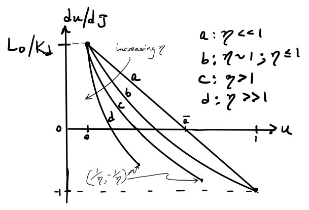
Figure 6: A phase portrait for the simple receptor-ligand binding depicts four cases: (a) (eta « 1) (ligand in excess), (b) (eta approx 1) with (eta le 1), (c) (eta > 1) and (d) (eta » 1). For each (eta), a curve is drawn spanning the physically-relevant domain for (u). All curves have the same y-intercept, (L_o/K_d).
We have dealt with the case where ligand is vastly in excess (\(\eta «1\)), and for reference, the associated curve (a) on the phase portrait is shown in Figure 6. The line is drawn based on Eq. \eqref{modelLexcess}.
When \(\eta \approx 1\), ligand and receptors are at comparable levels, and we use the non-linear model Eq. \eqref{modelLdepletion}. Still, as long as ligand outnumbers receptors (\(\eta \le 1\)), it remains possible, numerically speaking, for all receptors to bind ligand. Since the fraction of bound receptors (\(u\)) can reach a maximum of 1, the curve on the phase portrait considers the full domain \(0 \le u \le 1\). As depicted in Figure 6, the curve (b) is a concave-up parabola as defined by the second-degree polynomial in \eqref{modelLdepletion}, with \(du/d\tau|_{u=0} = L_o/K_d\) and \(du/d\tau|_{u=1} = -1\).
When \(\eta > 1\), more receptor is available than ligand. Thus, even when all ligand is bound, a fraction of receptors will remain unoccupied. The fraction of receptors in a ligand-bound state (\(u\)) can never reach 1. The maximum number of complexes is based on the amount of limiting reagent, the ligand: \(C_\mathrm{max} = N_{Av} V L_o / n\). Thus, the upper limit of \(u\) is \(C_\mathrm{max}/R_T = 1/\eta\) at which \(du/d\tau = -1/\eta\) according to Eq. \eqref{modelLdepletion}, as shown on curves (c) and (d) in Figure 6. The more \(\eta\) increases above a value of 1, the further left the parabolic curve on the phase portrait shifts.
Using the phase portrait, we can determine how the steady-state fraction of receptors in the bound state (\(\overline{u}\)) depends on the value of \(\eta\). The value of \(\overline{u}\) is greatest when \(\eta « 1\). As \(eta\) increases closer to 1 and then exceeds beyond 1, \(\overline{u}\) progressively decreases. The qualitative trend is sketched below (Figure 7).
Figure 7: The dependence of steady-state fraction of receptors bound to ligand ((overline{u})) on (eta). The value of (overline{u}) is obtained from the intersection of the phase portrait with the x-axis in Figure 6.
We can also use the phase portrait to better understand how \(u\) changes over time and its dependence on \(\eta\) (Figure 8). At initial time, \(u = 0\). The phase portrait shows that the initial rate of complex formation is \(L_o/K_d\) regardless of the value of \(\eta\). However, once \(u\) increases past its initial value, the value of \(du/d\tau\) is greatest when \(\eta « 1\), the trajectories on the time-course for \(\eta«1\) rise more rapidly than than do those for \(\eta \approx 1\) or for \(\eta > 1\). Furthermore, we know from our earlier analysis of steady-state, \(u\) plateaus to a higher value of \(\overline{u}\) when \(\eta «1\).
Figure 8: Dynamics of receptor-ligand binding for different values of (eta). The curves are marked (a)-(d) to correspond to the (eta) values shown in Figure 6.
14.3 Exercise
Above, we considered how changes in \(\eta\) affect the steady-state and dynamics of receptor-ligand binding (Figures 7 and 8, respectively). The analysis assumed that we hold fixed the other dimensionless parameter in the system, \(L_o/K_d\).
Here, we flip the scenario. For a fixed value of \(\eta \approx 1\), construct plots of the steady-state and dynamics of \(u\) for different values of \(L_o/K_d\).
15 The rate-limiting step: simplifying models of reaction systems
We have developed models of small systems of two or three elementary reactions. Even for such simple systems, it is evident that models can become intractable to analytical solutions. The challenge is magnified in biological systems. Biological processes, such as metabolism, signaling or gene regulation, typically involve large networks of reactions. It is therefore extremely useful to learn strategies to simplify dynamical reaction models and to become familiar with situations in which these simplications can be applied.
An important principle for simplifying models of reaction dynamics is the concept of a rate-limiting step. It is easily appreciated by considering a commonplace process that involves multiple steps. For example, consider a subway train transiting through a station. The transit comprises multiple steps: the train stops, doors open, passengers get off, new passengers get in, doors close, green light is given, train leaves. During evening rush hour at downtown stops, loading passengers is the rate-limiting step. However, if a jammed door fails to close, that step becomes rate-limiting to the overall process. To the consternation of everyone who wants to get home, the time to unjam and close the door will dictate the dynamics of the overall process.
Applying this concept of a rate-limiting step can significantly simplify models of chemical reactions.
15.1 Revisit sequential reaction
Without assumptions
Recall the conversion of species A into a final product C through a sequence of reactions: \(\ce{A ->[k_1] B ->[k_2] C}\). With no prior knowledge of the speed of the two reactions, we previously modeled the sequence of first-order reactions without making any assumptions. We derived the following solutions for the dynamics of the concentration of each species:
\begin{align} A &= A_o e^{-k_1t} \\ B &= \frac{k_1}{k_2-k_1} A_o \left(e^{-k_1t}-e^{-k_2 t}\right) \\ C &= A_o \left(1-e^{-k_1t} - \frac{k_1}{k_2-k_1} \left(e^{-k_1t}-e^{-k_2 t}\right) \right) \end{align}
for the situation where only A is initially present at a concentration of \(A_o\).
The results show that the dynamics of this system depends on both \(k_1\) and \(k_2\). As time progresses, concentrations of species change exponentially. How quickly these changes occur are dictated by \(e^{-k_1t}\) and \(e^{-k_2t}\). Thus, both reactions contribute to system dynamics.
Suppose one rxn is slow (\(k_1 « k_2\))
What if, however, one reaction is very slow? Suppose the first reaction occurs slowly compared to the second. That is, \(k_1 « k_2\). In this case, \(e^{-k_2t}\) will decay rapidly to zero and can be ignored relative to \(e^{-k_1t}\). The simplified solutions are:
\begin{align} A &= A_o e^{-k_1t} \\ B &\approx \frac{k_1}{k_2} A_o e^{-k_1t} \label{eq:qssaB}\\ C &\approx A_o \left(1-e^{-k_1t} - \frac{k_1}{k_2} e^{-k_1t} \right) \nonumber \\ &= A_o \left(1 - \left(1+\frac{k_1}{k_2}\right) e^{-k_1t} \right) \nonumber \\ &\approx A_o \left(1 - e^{-k_1t} \right) \label{eq:qssaC} \end{align}
where we have used \(k_2-k_1 \approx k_2\) and \(1 - k_1/k_2 \approx 1\).
Note that the dynamics of the system now depends only on the rate constant of the slow step — the rate-limiting step. As time progresses, the concentrations of all species evolve according to \(e^{-k_1t}\), the rate constant of the first slow reaction. Exponentials with \(k_2\) are eliminated.
While \(k_2\) does not influence the dynamics of the system, it does impact the magnitude of \(B(t)\). The rate constant appears in the coefficient to the exponential in \eqref{eq:qssaB}. It is especially instructive to rewrite \eqref{eq:qssaB} as:
\begin{equation} B \approx \frac{k_1}{k_2}A \label{eq:qssaBwrtA} \end{equation}
Because \(k_1/k_2 « 1\), it is evident that the concentration of B will be a small fraction of \(A\). The low concentration of B relative to A is consistent with the fact that even as B is generated gradually from A, it is consumed rapidly. Thus, B is a reactive intermediate.
The concept of quasi steady state
Importantly, Eq. \eqref{eq:qssaBwrtA} reveals B instantaneously tracks A. The concentration of B at every moment in time is directly proportional to the concentration of A. As the concentration of A changes, B changes immediately alongside.
Why does B track A so closely? The reason is not that B is achieving equilibrium with A. In fact, the conversion of A to B is irreversible. B tracks with A because B is immediately consumed in the next reaction. The second reaction is so fast that the concentration of B reaches its new level instantly.
This property of B to instantly adjust to changes in A implies that at every moment in time, B achieves a steady state. This notion of steady state should not be confused with the standard concept of steady state. We are not suggesting that the concentration of B does not change in time. Indeed, Eq. \eqref{eq:qssaBwrtA} tells us explicitly how the concentration of B changes in time. B exhibits the same time-dependence as A.
Steady state in this situation refers to a momentary phenomenon. As the concentration of A changes, at every moment in time, B immediately achieves steady-state. When A changes again in the next moment, B again immediately attains a steady-state. This notion of instantaneous or moment-by-moment achievement of steady-state is referred to as quasi steady state to distinguish it from the standard notion of steady-state.
15.2 Quasi steady state assumption (QSSA)
When a species is a reactive intermediate — it is produced slowly and consumed rapidly — the Quasi Steady State Assumption (QSSA) is used to approximate its dynamics. For the case of a sequential reaction \(\ce{A ->[k_1] B ->[k_2] C}\) with \(k_1 « k_2\), B is a reactive intermediate, and we apply QSSA to model the dynamics of B:
\begin{equation} \frac{dB}{dt} = \mathrm{rate\ of\ B\ production} - \mathrm{rate\ of\ B\ consumption} \approx 0 \label{qssa} \end{equation}
Because B is at quasi steady state, the processes governing the production and consumption of B balance out rapidly at every moment in time. The condition expressed in Eq. \eqref{qssa} holds at every moment in time.
Applying Eq. \eqref{qssa} does not mean that the concentration of B is constant with time. We expand \(dB/dt\) as follows:
\begin{align} \frac{dB}{dt} &= -k_1 A + k_2 B \approx 0 \\ B &\approx \frac{k_1}{k_2} A \label{applyQssaB} \end{align}
Note that applying QSSA leads us directly to our earlier observation that B tracks A (Eq. \ref{eq:qssaBwrtA}). The major difference here is that using QSSA, we arrive at the result with just simple algebra (Eq. \ref{applyQssaB}) without having to solve a system of differential equations.
The dynamics of A, B and C is quickly solvable, with B assumed to be at quasi steady state. We model the dynamics of A as before
\begin{equation} \frac{dA}{dt} = - k_1 A \end{equation}
to find
\begin{equation} A = A_o e^{-k_1 t} \end{equation}
From \eqref{applyQssaB}, we find that
\begin{equation} B = \frac{k_1}{k_2} A_o e^{-k_1 t} \end{equation}
Finally, the species balance is used to find C, noting that \(k_1/k_2 « 1\):
\begin{align} C &= A_o - A - B \\ &= A_o \left( 1 - \left( 1 + \frac{k_1}{k_2} \right) e^{-k_1 t} \right) \\ &\approx A_o \left( 1 - e^{-k_1 t} \right) \end{align}
15.3 Rapid equilibrium assumption (REA)
In some scenarios, the relatively fast reaction is reversible. For example, suppose the conversion of A to C involves a rapid reversible step in which A forms B:
\begin{align} \begin{split} \ce{A & <=>[k_f][k_r] B} \mathrm{\ (fast)} \\ \ce{B & ->[k_2] C} \end{split} \label{rx:rea} \end{align}
In this scenario, the rate-limiting step in the production of C is the second reaction. The quicker first step is achieves rapid equilibrium.
Rapid equilibrium does not mean that concentrations of A and B do not change over time. After all, the concentration of B cannot be constant in time, as B is converted slowly to C in the next step. That the first reaction is fast and achieves rapid equilibium means that as B is gradually depleted to form C, A is instantaneously converted to B in a manner that maintains an equilibrium ratio of A to B at each moment. Thus, depletion of B over time will drive forward the conversion of A. Thus, the concentration of all species do change over time.
The first reaction achieves rapid equilibrium every instant in time. Even as conditions change (at a rate determined by the slow second reaction), the first reaction quickly equilibrates to the new situation. Thus, the Rapid Equilibrium Assumption (REA) stipulates that
\begin{equation} K = \frac{k_f}{k_r} \approx \frac{B}{A} \label{reaConstraint} \end{equation}
where \(K\) is the equilibrium constant for the first reaction. Note that the concentrations in Eq. \eqref{reaConstraint} do not refer to concentrations of A and B at equilibrium. Eq. \eqref{reaConstraint} asserts that the concentrations of A and B at every moment meet the equilibrium constraint.
On your own, develop the model for the system \eqref{rx:rea} without the simplification afforded by REA. The practical value of REA should be apparent!
16 Enzymes: an introduction
Enzymes are biological catalysts. They make reactions go faster. Enzymes reduce the activation energy (\(E_a\)) for converting substrate (reagents) to product. By reducing \(E_a\), the rate constant is increased and the reaction proceeds more quickly than in the absence of enzyme.
Enzymes do not alter the \(\Delta G_R^o\). Thus, enzymes have no effect on making a reaction more or less favorable from an equilibrium perspective.
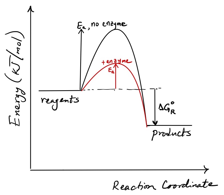
Figure 9: The effect of enzyme on the reaction coordinate diagram. An enzyme lowers the activation energy of a reaction but does not affect the standard-state Gibbs free energy of reaction.
A reaction can strongly favor product at equilibrium but be extremely slow to reach that equilibrium. Previously, we learned that a reaction that is highly exogernic (\(\Delta G_R^o \ll 0\)) strongly favors product at equilibrium. Its equilibrium constant is much larger than 1. However, this tells us little about how long it takes to make product.
The classical example is production of ammonia from hydrogen and nitrogen. With \(\Delta G_R^o = -32.8\) kJ/mol at 298 K, equilibrium strongly favors formation of ammonia; however, the reaction yields no appreciable product because of the high activation energy (\(E_a\)) of the reaction. Without a catalyst, the industrial process of producing ammonia would be hopeless.
Living systems hinge on dynamics, and therefore, rely on enzymes to reduce the activation energy and make reactions go faster.
Enzymes are not modified by reaction. Enzymes interact with and form a complex with substrate(s). At the end of the reaction, a product is released and the enzyme is recovered. Thus, over time in a reaction volume, a single enzyme molecule successively catalyzes the conversion of many substrate molecules into product.
16.1 The overall reaction and the elementary mechanisms
The main question in front of us is to predict how fast the reaction proceeds in the presence of enzyme. To tackle this question, we need to consider the elementary reactions by which the overall reaction is achieved. The overall reaction is:
\begin{equation} \ce{S ->[E] P} \end{equation}
with E written above the arrow to indicate that it is neither reagent nor product in the classical sense.
What are the elementary steps or mechanisms by which the overall reaction is achieved? A common method to model enzyme-substrate reactions is the Michaelis-Menten model. In this model, the enzyme interacts and binds with substrate to form an enzyme-substrate complex (ES). The enzyme modifies the substrate to which it is associated and releases the product in the final catalytic step. The elementary mechanisms are:
\begin{align} \ce{E + S & <=>[k_f][k_r] ES} \\ \ce{ES & ->[k_2] E + P} \end{align}
The rate constant for the catalytic step is also referred to as \(k_{\mathrm{cat}}\). Next, we use this model of elementary reactions of an enzyme-substrate reaction to determine how quickly product (P) is formed.
Copyright ©2018 Anand Asthagiri. All rights reserved
-
We will define terms like equilibrium more formally later. ↩︎
-
Note this says ‘bimolecular’: two reagents come together to form products. Whether it is biomolecular are not is inconsequential for this generic example. ↩︎
-
Very rarely, elementary steps involve three reagents. ↩︎
-
These steps are not detailed here, but we will discuss them later. ↩︎
-
Notation: Hereon, concentration will be written without the brackets. Thus, \([C]\) is simply \(C\). Following standard convention, the concentration \(C\) is italicized, whereas the name of species C is not. ↩︎
-
See perspective written by Judith Herzfeld in Atlas of Science, Apr 2018 and her work with colleagues published in Bai et al., Chem. Sci. (2017) 8: 4203-4210. ↩︎
-
The final step is in fact two steps: pure species \(i\) is brought from \(P^o\) to reaction pressure \(P\) and next taken from pure substance into the reaction mixture with other species. When dealing with an ideal gas in an ideal mixture, the contribution to Gibbs free energy is \(RT \ln{p_i/P^o}\) where \(p_i\) is the partial pressure in the mixture. To capture deviations from ideal behavior, the concepts of activity \(a_i\) and fugacity (\(f_i\)) are introduced. It is beyond the scope here to detail the theoretical underpinnings and the forms of models for activities and fugacities. ↩︎
-
It can be helpful to use Eq. \eqref{conservHb} to rewrite Eq. \eqref{conservO2} as \(\Delta n_{\ce{O2}} = - \Delta n_{\ce{Hb1}} - 2 \Delta n_{\ce{Hb2}} -3 \Delta n_{\ce{Hb3}} - 4 \Delta n_{\ce{Hb4}}\). A loss of one \(\ce{Hb4}\) is a gain of four \(\ce{O2}\). ↩︎
-
We could have picked another pair. ↩︎
-
In some literature, \(n/V\) is subsumed into a single parameter \(n\) or \(n_c\), a volumetric density of cells. ↩︎
-
Also equilibrium for this closed system ↩︎
-
The terms lost or depleted refer to a decrease in free ligand. The amount of total ligand is, of course, not lost; it is conserved. ↩︎